Article of the Month - November 2020

A method to estimate a best fit trajectory from multiple individual trajectories

Ola Øvstedal, Norway

SUMMARY

In applications like extracting hiking trials from crowd sourced data, collecting trajectories describing animal movement or precise mapping of road lines, there are multiple trajectories, obtained from e.g. Global Navigation Satellite Systems (GNSS), that describe the same physical path. Due to e.g. observation techniques, occasional observational blunders and difficulty in identifying exactly the same physical path, individual trajectories will normally differ from one another. This paper proposes a method on how to estimate a best fit trajectory based on available individual trajectories. The precision of the estimated trajectory is quantified in form of standard deviations. Occasional observational blunders and failure in following the same physical path are addressed through statistical testing. A priori stochastic information regarding the individual trajectories is utilized in a weighting scheme. The proposed method is first verified using a simulated dataset. Results from processing of a relatively complex dataset stemming from individual runs with a GPS multi-sport watch, point out some advantages and drawbacks of the method. The method appears to handle well both observational blunders and changing requirements regarding following the very same physical path during data collection. Detection and subsequent deletion of erroneous observations might however introduce small jumps along the estimated trajectory. Depending on the applications, the effect of occasional small jumps can be handled by post smoothing.

1. INTRODUCTION

GNSS (Global Navigation Satellite Systems) like GPS (Global Positioning System) is frequently used in kinematic mode to obtain trajectories in the form of temporally ordered sequences of geographic coordinates. Depending on factors like hardware, software, observation- and processing techniques, satellite geometry and observational errors from e.g. atmosphere and multipath (e.g. Teunissen & Montenbruck, 2017) positional accuracies ranging from centimeter to several tens of meters can be achieved.

Precise georeferencing of centerlines of roads is an example where a high accuracy is required while an accuracy of a few meters is sufficient for e.g. hiking trials. Most users require that quality numbers should accompany the coordinates, e.g. standard deviations or Dilution of Precision (DOP). If a trajectory is measured only once, statistical information from the GNSS-processing can supply such quality information. As with nearly all measuring techniques however, observational blunders in the form of outliers will occasionally lead to erroneous coordinates. An approach to overcome and reduce the effect of outliers is to repeat the measurements leading to a redundant set of trajectories. The problem then arises on how to estimate an optimal trajectory based on individually measured trajectories as well as how to compute corresponding quality numbers.

Each trajectory will not have identical sampling locations as common tie points are normally not available. Each trajectory is obtained individually and differences regarding start and stop of each trajectory, epoch interval, speed and occasionally missing epochs make the estimation of an optimal trajectory complicated.

Existing methods like manual methods, Mean and Median methods (Buchim et al., 2013) and Dynamic Time Warping (Vaughan & Gabrys, 2016) have different strengths and weaknesses regarding different sampling characteristics.

The current paper proposes a method based on traditional least squares parameter estimation. In a first step temporarily ordered point clouds containing coordinates from each individual trajectory are identified. For each point cloud, network adjustments and analyses are carried out where outliers are identified using multiple t-testing. Final coordinates are estimated using the remaining healthy observed coordinates. Precision numbers are computed in the form of covariance matrices or standard deviations. The method could find use in extracting e.g. popular hiking trials from crowd sourced data, collecting trajectories describing animal movement or in precise mapping av road lines.

Section 2 gives a very short review of GNSS positioning in kinematic mode highlighting different coordinate systems and reference frames as well as stochastic information accompanying the coordinates. Section 3 is on the formation of discrete point clouds while section 4 gives the theoretical outline of the proposed method. Section 5 presents processing results using trajectories from a simulated dataset and section 6 presents results from a more complex scenario where individual trajectories have been measured using a GNSS multi-sport device. Discussion and some suggestions for future work are presented in section 7 while section 8 contains conclusions.

2. GNSS KINEMATIC POSITIONING

In the GNSS device or GNSS software, raw observations in the form of distance measurements between the GNSS receiver antenna and antennas of GNSS satellites are used to estimate three-dimensional receiver coordinates (x,y,z) along with nuisance parameters such as e.g. receiver clock biases (e.g. Teunissen & Montenbruck, 2017). Estimated receiver coordinates are Earth Centered Earth Fixed (ECEF) coordinates given in the reference frame defined by the coordinates of satellites and eventual differential reference stations. Using a handheld GPS-receiver, satellite coordinates are normally obtained from the broadcasted navigation message and coordinates are then referred to WGS84. Broadcasted navigation messages from other GNSS-systems such as GLONASS, Galileo and Beidou are using reference frames which are nearly identical to ITRF (International Terrestrial Reference Frame), which again is nearly identical to WGS84 (e.g. Teunissen & Montenbruck, 2017).

For most geomatic applications, three-dimensional Cartesian xyz-coordinates in the ECEF coordinate system are converted to planimetric coordinates (North, East) and height (e.g. Hofmann-Wellenhof et al., 2008). The conversion from xyz-coordinates to North-, East-, height-coordinates is a two-step procedure. The first step involves conversion to latitude, longitude and ellipsoidal height related to a reference ellipsoid. The last step involves conversion from latitude and longitude to Northing and Easting in the mapping plane by applying an appropriate mapping projection. Ellipsoidal heights are converted to gravity based heights using corrections in the form of e.g. geoid heights obtained from a geoid-model. If working with coordinates in a regional reference frame, e.g. the European ETRF89, receiver coordinates in the global WGS84 or ITRF should be transformed to the regional reference frame. The transformation involves the time difference from the epoch of observation to the reference epoch of the regional reference frame as well as spatial differences between the reference frames at the corresponding reference epochs (e.g. Nørbech & Plag, 2002). Most national mapping agencies supply transformation formulas and software to transform and to convert GNSS-coordinates obtained from single point GNSS positioning to the national reference frame.

Along with estimated receiver coordinates, accompanying covariance-matrices are initially available from the GNSS processing. The initial 3x3 covariance matrices for Cartesian ECEF-coordinate can be converted to 3x3 covariance matrices for North-, East- and height coordinates using the general law for error propagation (e.g. Ghilani, 2017). It should be pointed out that some GNSS devices and software output full three-dimensional covariance information, some output standard deviations only (ignoring correlations between estimated coordinates) and some do not output any quality measures at all. When working with trajectories, the height coordinates are normally ignored as only horizontal coordinates are of interest. Covariance matrices accompanying North- and East coordinates are then reduced to 2x2-matrices.

3. IDENTIFICATION OF DISCRETE POINTS CLOUDS ALONG THE TRAJECTORY

The proposed method is based on the fact that all points along a trajectory have corresponding neighbor points in accompanying trajectories. Our criteria for selecting corresponding neighbors for a point in one trajectory is based on the minimum Euclidean distance to points in the other individual trajectories. Typical sampling interval of a GNSS-device is 1 second. The spatial distance between adjacent points along a trajectory then depends on speed, typically 1.4 m/s for a pedestrian (Levin & Norenzayan, 1999) and 13.9 m/s for a car travelling at a speed of 50 km/h. To minimize the effect of sampling rate on the choice of nearest neighbor, the spatial density of points along each trajectory can be increased by e.g. linear interpolation. For trajectories sampled by a handheld GNSS device with a horizontal accuracy of 5 m (one sigma), a spatial distance of e.g. 0.05 m between points along the trajectory will minimize the effect of sampling rate on choice of neighbor points.

Following a densification of each individual trajectory, one trajectory is selected as reference trajectory and for each point, a search is carried out to find nearest neighbors in accompanying trajectories.

Denoting the number of individual trajectories m and the spatial distance between points along each trajectory d_dist, the clustering algorithm will output a series of point clouds along the trajectory. Each point cloud consists of m points and the distances between point clouds are approximately d_dist.

The clustering process might be sensitive to the choice of initial reference trajectory. The search for nearest neighbors can therefore be iterated where e.g. weighted mean coordinates of each point cloud are used as reference in a re-search for the m closest neighbors. Subsequent re-clustered point clouds are then used to estimate and validate outliers and to estimate coordinates along the final trajectory.

4. ESTIMATION AND VALIDATION

4.1 Estimation of coordinates and standard deviations

The suggested approach is based on least squares parameter estimation (e.g. Ghilani, 2017). Independent estimation and analysis processes are carried out for each point cloud along the trajectory. The number of point clouds is denoted n and the number of points in each point cloud is m. Cloud number is also an epoch number and is indicated with subscript i, i=1,2,…., n. We use superscript j to indicate individual points in each point cloud, j=1,2,…., m. Unknown parameters for each point cloud are horizontal coordinates N_i and E_i. The coordinates of each point in the point cloud, N_i^j and E_i^j are treated as observations and the number of observations in one point cloud is thus 2m. The observations are assigned weights using 2x2 covariance matrices, Σ_i^j, accompanying each tuple of observed North- and East coordinates. 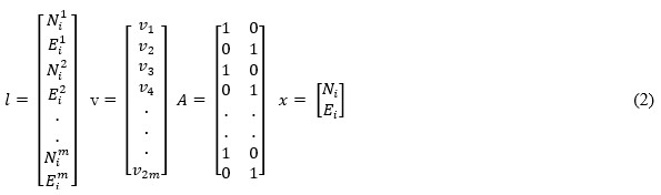In the functional model, we express the observations as a function of the unknown parameters.

, where vector l contains the observations in each point cloud, v is vector with residuals, A is design matrix and x is vector with unknown parameters.

Applied to our case, we get

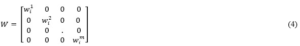
Due to lack of information, we ignore temporal correlations between subsequent coordinate pairs in the stochastic model. If 2x2 covariance matrices, Σ_i^j, for each pair of individual coordinates are available from the GNSS processing, weight matrices for each pair of observations are given by

The full weight matrix, W , is then a block diagonal matrix with epoch wise 2x2 matrices w_i^j along the diagonal.

The degrees of freedom, being the number of redundant observations, is r = 2m – 2 for each point cloud.

Applying the principle of least squares gives us the estimated parameters as

The vector with residuals is computed as

The standard deviation of unit weight is then

And standard deviations of estimated parameters can be computed as

Where q₁₁ and q₂₂ are respective diagonal elements in the cofactor matrix Q

The covariance matrix of estimated coordinates is given by

As a measure of goodness of fit, the estimated standard deviation of unit weight, s₀, can be tested against the a priori value, σ₀, using the standard Chi-square test. Normally σ₀=1 is used as a priori value.

If the computed χ2 is greater than the tabulated value with r degrees of freedom and significance level of α (e.g. α=0.05), there is a significant difference between a priori- and estimated standard deviation of unit weight.

4.2 Extending the model to include outliers

Several methods have been developed in an effort to reduce the influence of observational blunders. Traditional approaches for geodetic measurements are based on attempts to detect, identify and remove outliers (e.g. Baarda, 1968; Pope, 1976) or robust estimation designs to mitigate the influence of outliers on the parameter estimates (e.g. Huber, 1981). In this work, a relatively simple approach based on multiple t-testing is presented (Pelzer, 1985; Asplan Viak, 1994). For each single observation in the point cloud, we estimate an outlier as one additional unknown parameter in the model described above. The vector with observations, l , as well as the weight matrix, W , remain as above while the design matrix A is extended with a new column to accommodate the new outlier parameter.

The vector with unknowns is now

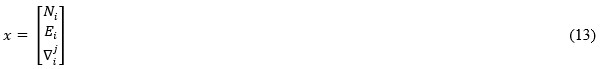
Where is the estimated outlier for observation number j in the point cloud.

For the first observation (j=1), A is

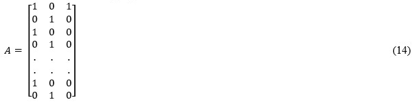
Estimated parameters, residuals and standard deviations are computed as given by eq.5 - eq.7. Standard deviation for the estimated outlier is computed with

Where q₃₃ is the third diagonal elements in the cofactor matrix Q (eq. 10). For each observation, the number 1 in third column of design matrix A is in a sequential manner interchangeably moved to each observation to be tested, j=1,2,3,…,2m. A program run is carried out for each observation (j), where estimated outliers with corresponding standard deviations,, are used to compute t-values

The t-values are T-distributed with r = 2m-3 ; degrees of freedom. As the estimated outlier can have both positive and negative signs, this is a two-sided t-test. Furthermore, when testing with a total significance level of α (e.g. α = 0.05) the significance level of each individual test has to be adjusted due to multiple testing. Assuming independent observations, the significance level of each individual test, j, can be computed by

If the number of observations to be tested is large (e.g. 2m >30 ), a value of αj=0.001 is frequently used.

The outlier estimation and testing approach is a nested iterative process. First the most extreme outlier is identified as being the associated with the largest computed . This is then checked against the tabulated T-value using r degrees of freedom and significance level of . If the most extreme outlier is significantly different to zero, the associated observed point is removed and the whole procedure is repeated for the remaining j=1,2,3,…,(2m-2) observations (e.g. Ghilani, 2017).

The whole procedure is repeated until the most extreme outlier value is not significantly different to zero. Final estimates and standard deviations for coordinates are estimated using the remaining observations.

Only the outlier parameter and associated standard deviationare required in the search for outliers. To speed up the computations in an operational software, the somewhat naive approach of estimating the full set of unknowns and standard deviations for every observation to be tested can be replaced by an approach based on Cholesky decomposition and back solution of an extended system of equations (e.g. Asplan Viak, 1994 ; Leick et al., 2015).

5. SIMULATED TRAJECTORIES

In this section the proposed method is used to estimate a trajectory based on a simulated dataset. A “true” reference trajectory is made up from line-segments connecting 11 control points, see figure 1. Distances between adjacent control points are approximately 7 meters. Four simulated trajectories are now computed.

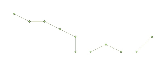
Figure 1. True trajectory. Approximate distances between adjacent points are 7 meters.

Around each of the 11 control points, coordinates of four randomized points are generated using the Matlab “randn-function” (Matlab Release 2018a, 2018). The Matlab “randn-function” returns normally distributed random numbers. A standard deviation of 1 m is used in the generation of each randomized coordinate, North and East respectively. Line-segments connecting individual points in each cluster finalize the four simulated trajectories, see figure 2.

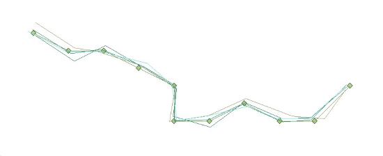
Figure 2. Four simulated trajectories shown together with the true trajectory.

We now attempt to reconstruct the reference trajectory from the four simulated trajectories. Along each simulated trajectory, densified trajectories are generated using linear interpolation. Intermediate distances along the four resampled trajectories are 0.05 m. As described in section 3, the minimum Euclidian distance principle is now used to identify a total of 2213 discrete point clouds along the resampled trajectories. The estimation and validation scheme described in section 4 is used to estimate a best fit trajectory based on the four simulated trajectories. Figure 3 shows the original reference trajectory along with the estimated trajectory from a program run where the outlier detection algorithm has not been applied. As seen from figure 3 along with figure 2, the estimated trajectory fits the reference trajectory better than each of the individual trajectories.

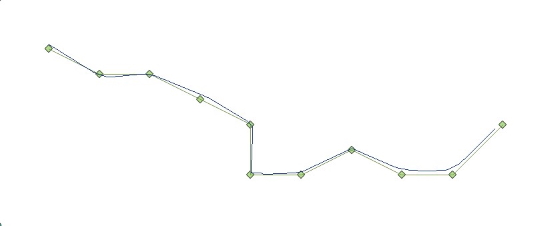
Figure 3. Trajectory estimated without application of outlier detection, shown together with true trajectory.

Figure 4 shows the estimated trajectory stemming from a program run were also the outlier detection algorithm was applied. 261 of the total 8852 “observed” coordinate-pairs (2.9 %) were detected as outliers and omitted in the estimation of the final estimated coordinates that constitute the trajectory. It can be observed that the occasional detection of outliers along the estimated trajectory results in small jumps.

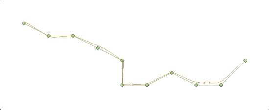
Figure 4. Trajectory estimated with application of outlier detection, shown together with true trajectory. Occasional small jumps can be seen along the estimated trajectory.

Table 1 presents some details concerning the estimated standard deviations for estimated coordinates along the trajectory.

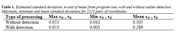
In this simulated dataset, estimated North- and East coordinates have identical standard deviations. As the same random algorithm is used in the simulation of both North- and East coordinates, the associated estimated standard deviations have the same magnitude. As expected, the minimum and mean of estimated standard deviations are smallest for the program run with outlier detection.

5. TRAJECTORIES COLLECTED WITH A GARMIN FORERUNNER 910XT MULTI SPORT DEVICE.

A Garmin Forerunner 910XT Multi Sport device is used to log positions while running a loop of approximately 4.7 kilometer, see figure 5. The device operated in the default data recording mode of smart recording (Garmin, 2014). In smart recording mode, positions are recorded based on a proprietary algorithm for change in direction, speed or hearth rate. The data files are then smaller compared to the alternative setting of recording positions every 1 second. Inspecting the resulting data files, reveals that the recording interval vary between 1 second and ca. 10 seconds. With an average pace of approximately 6 minutes per kilometer, there is a recorded position approximately every 2.8 – 28 meter. The majority of the recordings are sampled approximately every 2-3 seconds / 5.6-8.4 meter respectively.

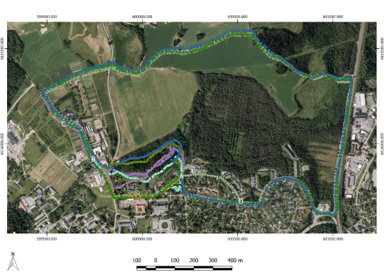
Figure 5. Plot of eight individual trajectories. Locations mentioned in the description of artifacts a, b, c and d are shown with white capital letters.

A total of eight runs started and ended at approximately the same location A, see figure 5. The eight trajectories are run clockwise and distributed in time over a period of more than one year, see table 2

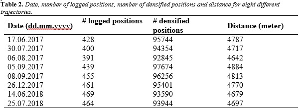
Some artifacts can be seen from figure 5 and are due to:

A. It is a well-known issue with the Garmin Forerunner 910XT device that the first recorded positions occasionally have errors of several tens of meters. The possibility of erroneous first positions is higher if the device has not been used for a while.

B. From the starting point A to approximately point B, the runner chose three different paths. Four of the runs started off in a south-west direction, following the road. Two of the runs first followed the road in a northern direction from the starting point A before turning in a western direction following a foot-path through the forest. Finally two of the runs selected a foot-path that goes between the other two initial choices.

C. From approximately point B to approximately point C, the runs chose slightly different paths. Some runs followed the road while the others followed a footpath. The footpath runs approximately 10-30 meters to the right of the road. This is in an area with tall threes and thick foliage.

D. In the end of the loop from point D, returning to the approximate start- and end-point A, seven of the runs followed the same path. One run did however choose a complete different road to the north of the other runs.

In the data processing, the artifacts concerning some of the individual trajectories are not taken into concern, and the proposed method is used to estimate coordinates for a best fit trajectory along with quality data in the form of estimated standard deviations (eq. 5 and eq. 8-9). The recorded data are downloaded from the device and converted to files with coordinates in the ETRF89 reference frame using the UTM map projection in zone 32. The Garmin Forerunner 910XT device does not provide any quality measures of logged positions. Assuming equal accuracy for independent North- and East coordinates and an horizontal accuracy of approximately 5 meters (e.g. van Diggelen & Enge, 2015), a priori standard deviations σN,GNSS and σE,GNSS are both assigned a value of 3.5 meter. To take into account that different runs occasionally follow slightly different paths, e.g. left side of a road on some runs and right side of the same road on other runs, the standard deviation designated each observed coordinate is augmented with a term that takes offsets between physical paths into account. Assuming that errors are random and that GNSS errors are independent from track-offset errors, a priori standard deviations for track-offsets, σN,Track and σE,Track are used in the propagation of a priori final variances:

Where are a priori variances for North- and East coordinates respectively and subsequently used in the weighting scheme by populating the 2x2 covariance matrices, , in eq. 3. In the present estimation and analysis, are both assigned values of 2 meters.

Each trajectory is first resampled to a distance of 0.05 m between adjacent points. The minimum Euclidian distance principle as described in section 3 is then used to identify a total of 94 354 discrete point clouds along the trajectory before the estimation and validation scheme suggested in section 4 is used to estimate the final trajectory. A program run without the outlier detection algorithm averages out the effects of the artifacts mentioned above and estimated coordinates and trajectory from this approach is not shown here. In figure 6, the background orthophoto is removed and shows the estimated coordinates from a program run were the outlier detection algorithm is applied. A first glance at figure 6 reveals two interesting observations:

In the beginning of the loop, from the starting point A to approximately point B, there is only small segments of estimated coordinates as the outlier detection has rejected most of the observed coordinates. Estimated coordinates for the small segments in this first part have associated standard deviations of several tens of meters.
In the end of the loop, from point D to the start- and end-point A, the estimated trajectory follows the main path defined by seven of the runs. The deviated path of the one single run is rejected by the outlier detection approach.

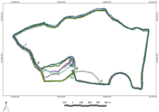
Figure 6. Plot of estimated trajectory from a program run with outlier detection algorithm applied. The estimated trajectory is shown as a thin black line together with the eighth individually observed trajectories. Compared with figure 5 the background orthophoto is removed in order to better see poorly estimated segments. Locations mentioned in the description of artifacts a, b, c and d are shown with capital letters.

The combined effect of artifacts a, b and c, mentioned above, is that one common trajectory is not justified for the start segment from point A to point B and further on to point C. As seen in figure 6, the proposed estimation and validation scheme has nevertheless produced short segments of a trajectory in this first part. The reason why not all observations have been rejected in this part, is that the outlier detection approach has not been able to distinguish between “good observations” and “bad observations”. All observations have passed the t-test, but estimated coordinates are associated with very high standard deviations. In the final step, a filter based on the outcome from the test of estimated standard deviation of unit weight (eq. 12) is therefore used to reject poorly estimated coordinates.

Figure 7 shows the final accepted trajectory with a thin line. Segments filtered out by the Chi-square test are marked with thicker black dots.

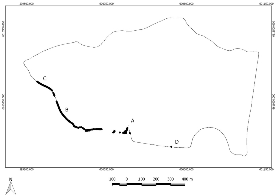
Figure 7. Plot of estimated trajectory from a program run with outlier detection algorithm applied. Accepted trajectory with a thin line and segments rejected in the Chi-square test with thicker black dots. Locations mentioned in the description of artifacts a, b, c and d are shown with capital letters.

Concerning artifact d, the outlier detection algorithm effectively detected that the path selected by one run significantly diverges from the path selected by all the other runs. Table 3 gives maximum, minimum and mean standard deviations for estimated coordinates for accepted and rejected coordinates respectively. In the stochastic model, we have for the current dataset assumed that observed North- and East coordinates are independent of one another. Since there is no common information between estimated North- and East coordinates in the functional model, all standard deviations are then equal for estimated North- and East coordinates.

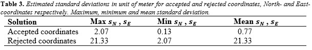
Figure 8 shows cumulative distribution plots of standard deviations for accepted and for rejected coordinates. For the accepted coordinates, the largest standard deviation is approximately 2.1 m, and 95% of standard deviation are smaller than 1.5 m. For the rejected coordinates, the largest standard deviation is approximately 21.3 m, and 5% of standard deviations are larger than 20.2 m.

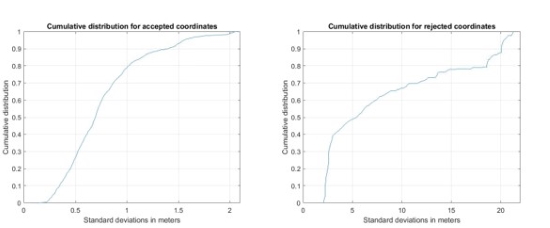
Figure 8. Cumulative distribution for North- or East-coordinates for accepted points left and rejected points right.

7. DISCUSSION AND SOME SUGGESTIONS FOR FUTURE WORK

Detection and removal of occasional outliers introduce sudden small jumps in the estimated trajectory, as seen in figure 4 in the section with the simulated dataset. Depending on the actual application, there can be a need to smooth out such inconsistences. The handling of practical aspects does also deserve attention, e.g.:

methods and techniques on how to fill in gaps in estimated trajectories,
interpolation techniques when densifying the original trajectories, e.g. linear interpolation or splines,
optimization of computational speed,
datasets with individual trajectories where some observers choose to go left of an obstacle, e.g. a lake, and other choose go right,
datasets with very curved trajectories,
datasets with nested trajectories.

Finally, alternative methods for dealing with outliers as well as the acceptance criteria for automatically rejecting segments with “bad” observations are interesting topics. E.g. when estimating the trajectory of centerlines of roads, a stricter acceptance criteria is required regarding choice of the same physical path than for e.g. hiking trials. This proximity requirement can for different applications be managed by tuning the augmentation of the a priori covariance matrices for observed coordinate (eq. 18). Assigning smaller track-offset terms (e.g. center lines of roads) will make the goodness of fit test (eq. 12) more sensitive to diverging paths than larger track-offset terms (e.g. hiking trials). How to assign proper track- offset values,, to take into account required proximity for individual physical paths should be further explored.

8. CONCLUSIONS

In this work, a method is proposed on how to automatically estimate one best fit trajectory from several individually measured trajectories. The proposed method uses a weighted least squares approach to take into account a priori accuracies and correlations of individual trajectories. An outlier detection algorithm based on multiple t-testing is used to isolate and omit bad observations. The outlier detection algorithm might also detect if any selected paths significantly deviates from other choices of paths. Remaining segments of bad observations or multiple choices of paths can be identified by applying a final filter based on a statistical test of goodness of fit.

The final product is a trajectory consisting of a temporally sequence of coordinates. Each estimated coordinate has an associated quality number in the form of a standard deviation. Due to erroneously observed coordinates or choice of multiple diverging paths during data collection, there might be gaps in the final trajectory. Eventual gaps can subsequently be flagged and give information on that additional measures must be used to finalize the trajectory. The proposed method can be applied to trajectories from different sources. E.g. trajectories in existing databases can be combined with newly observed trajectories. The difficult task then is how to assign proper a priori stochastic information to the different trajectories, ideally in the form of full variance-covariance information.

REFERENCES

Asplan Viak IT. (1994). Gemini Net/GPS-Brukerhåndbok. Asplan Viak Informasjonsteknologi A.S. (in Norwegian)
Baarda, W. (1968). A testing procedure for use in geodetic networks. Netherlands Geodetic Commission, Publications on Geodesy, New series Vol.2 No 5. Delft.
Buchin, K., Buchin, M., van Kreveld, M., Löffler, M., Silveira, R.I., Wenk, C., & Wiratma, L. (2013). Median Trajectories. Algorithmica, 66, 595-614.
Garmin, (2014). Garmin Forerunner 910XT Owners Manual. Garmin Ltd 2014, available from http://static.garmin.com/pumac/Forerunner_910XT_OM_EN.pdf, (accessed on 21.01.2019).
Ghilani, C.D. (2017). Adjustment Computations: Spatial Data Analysis. 6th. Edition, Wiley. Hofmann-Wellenhof, B., Lichtenegger, H., Wasle, E. (2008). GNSS – Global Navigation Satellite Systems. Springer.
Huber, P.J. (1981). Robust statistics. Wiley, New York. Leick, A., Rapoport, L., Tatarnikov, D. (2015). GPS Satellite Surveying, fourth edition. John Wiley Sons.
Levine, R.B., Norenzayan, A. (1999). The Pace of Life in 31 Countries. Journal of Cross-Cultural Psychology, Vol. 30, No. 2, 178-205.
Matlab Release 2018a. The MathWorks, Inc. (2018), Massachusetts United States, available from https://se.mathworks.com/help/matlab/index.html (accessed on 19.02.2019).
Nørbech, T., Plag, H.P. (2002). Transformation from ITRF to ETRF89(EUREF89) in Norway. EUREF Publication No. 12, Mitteilungen des Bundesamtes für Kartographie und Geodäsie, pp. 217-222. Verlag des Bundesamtes für Kartographie und Geodäsie, Frankfurt am Main.
Pelzer, H. (1985). Geodätische Netze in Landes- und Ingenieurvermessung. Vorträge des Kontakstudiums II. Wittwer Verlag. (in German)
Pope, A. (1976). The statistics of residuals and detection of outliers. NOAA Technical Report, NOS 65 NGS 1. Rockville.
Teunissen, P.J.G., Montenbruck, O. (2017). Springer Handbook of Global Navigation Satellite Systems. Springer.
van Diggelen, F., Enge, P. (2015). The World’s first GPS MOOC and Worldwide Laboratory using Smartphones, Proceedings of the 28th International Technical Meeting of The Satellite Division of the Institute of Navigation (ION GNSS+ 2015), Tampa, Florida, September 2015, pp. 361-369.
Vaughan, N., Gabrys, B. (2016). Comparing and combining time series trajectories using Dynamic Time Warping. 20th International Conference on Knowledge Based and Intelligent Information and Engineering Systems, KES206, 5-7 September 2016, York, United Kingdom, Procedia Computer Science 96, 465-474.

BIOGRAPHICAL NOTES

Ola Øvstedal is an Associate Professor at the Section of Geomatics, Faculty of Science and Technology, Norwegian University of Life Sciences. He received his PhD in geodesy in 1991. Current research interest are satellite positioning and estimation techniques. He is a national delegate to FIG Commission 5 “Positioning and Measurements”.

CONTACTS

Ola Øvstedal Section of Geomatics, Faculty of Science and Technology
Norwegian University of Life Sciences
P.O.Box 5003, N-1432 Ås, Norway
Tel: +47 67231549
Web site: https://www.nmbu.no/en