Methodological proposal for measuring and predicting Urban Green Space per capita in a Land-Use Cover Change model: Case Study in Bogota

Daniel Páez	Abbas Rajabifard	Joaquín Andrés Franco Gantiva

This paper was presented at the Commission 7 Annual Meeting in Bogota Colombia. It describes the problem of lack of sustainable urban planning and territorial ordinance plans which have led to nullification, fragmentation and reduction of green space and strategic ecosystems within cities.

SUMMARY

The lack of sustainable urban planning and territorial ordinance plans have led to the nullification, fragmentation and reduction of green space and strategic ecosystems within cities. A clear example of this problem is the city of Bogotá. Currently, Bogota has around 4 m2 of green space (GS) per capita, an amount significantly below the 10 m2 recommended by the World Health Organization (WHO). This research aims to establish how GS is distributed and relates to other land uses, transport infrastructure and other variables. For this purpose, ordinary least squares (OLS) and geographic regression (GWR) models were used. Both models are intended to determine the relationship at global and at neighbourhood scale between the GS per capita and other variables. Using Metronamica software and Information from 2005 and 2014, a 2040 greener scenario for the city of Bogota was developed. Results from this research highlighted the location of green space problems in Bogota. It has also opened the opportunity for decision-makers to understand in a quantitative way how GS is distributed and its benefits. Improve GS relationships is expected to support sustainable planning in large cities.

1. INTRODUCTON

Since the industrial revolution, most of the population growth has been concentrated in the cities. They have become supports of the modern economy and the centre of development for any country. This type of artificial ecosystem is characterized by their changeable and dynamic system that daily are consuming, transforming and releasing materials and energy (Bottalico, et al., 2016). This dynamism is correlated with increased production and consumption of goods, services and infrastructure. However, at the same time, it has led to greater land urbanization, landscape fragmentation, biodiversity loss, the creation of urban heat islands, increasing greenhouse gas emissions, increasing vulnerability to climate change events and the destruction of strategic or sensitive ecosystems (Norton, et al., 2015).

To reduce and overcome these issues many cities, from developed and developing countries, are evaluating mechanisms to plan and structure a more efficiently growth. Commonly four main principles are use: economic development, environmental equilibrium and sustainable development, transparent policies and government, and are focusing on cultural identity, factors that can be evaluated and grouped in a sustainability circle (James, Magee, Scerri, & Steger, 2015). This new city planning is becoming a stronger movement mainly in cities of developed countries, where planning policies are focused towards sustainable modes of transport, more compact and dense cities, efficient, greener and liveable for current and future generations (Gedge, 2015) & (Barbosa, et al., 2007) & (Demuzere, et al., 2014).

One of the main pillars of this new wave of urban planning thinking is the development towards environmental sustainability. This can be seen in several cities, mainly Europe and Asia (e.g. Vitoria-Gasteiz or Singapore). In this cities, they have focused their attention on generating and preserving all the potential of green and blue spaces (water bodies), in order to increase the quality of life of their citizens (Jim C. Y., 2004). This planning thinking enables Urban Green Infrastructure (UGI) to arise and can be interpreted as a hybrid infrastructure between old and new buildings with Green Space (henceforth as, GS) inside or in the border of the cities.

The UGI's have emerged as a tool to generate new GS or even to recover those that were lost. In turn, it has proven the benefits that this type of spaces provide, as they are not only part of the landscape, but also at the level of ecosystem services, valuation and capture of land value, tourism attractiveness, among others (Norton, et al., 2015) (Bolund & Hunhammar, 1999) (Jim & Chen, 2006). Also, these arise as an option in cities that are already consolidated and have a high population density, but lack GS or have a decrease of green areas. Given these conditions, these cities have a major vulnerability to the effects of climate change. The lack of these strategical areas generates a reduction in the land capacity of infiltration, changes in the underground water flow, an increase of removal in mass events and of the urban heat, a lack of tools to reduce or control air pollution, among others (Jo, 2002).

Furthermore, all the planners and the decision makers must take in consideration of the preservation and the greening of the city as a priority urban planning; not only to understand the causes and impacts which the urban sprawl brings but also the opportunities that new spaces can provide. Therefore, the current research aims to understand GS location based on its relationship with other land uses, transportation infrastructure, water bodies and other variables. Also, it is desired to identify which zones in a city lack of these spaces, in order to take actions to generate new green infrastructure, mainly parks, in these zones. The testing of this indicator will be applied in an existing model called “Bogotá Land Development (BoLD)” which was built by the group SUR in association with the French Development Agency (AFD, by their acronyms in Spanish and French) and uses a dynamic land cover change model based on a cellular automata (CA) software Metronamica.

2. BACKGROUND

Rapid urbanization in the last century has led to changes in GS inside or near the city. Urbanization has contributed to the disappearance of these spaces and ecosystems that have generated significant changes in the urban climate dynamics. Today natural land surfaces and urban vegetation has been replaced by surfaces and constructions that have the ability to absorb solar radiation. This has led to the generation of different microclimates in urban areas (Norton, et al., 2015). The lack of GS led to substantial changes in the infiltration and retention capacity of the soil, altering the flow of groundwater (Demuzere, et al., 2014). These changes have led to a gradual increase of temperature in urban areas, which is reflected by an increase in forest fires events, landslides and the reduce disposal of urban water resources, that finally leads to an increased vulnerability for climate change at local level.

At the same time, urbanization patterns are always associated with the fragmentation and nullification of strategic ecosystems. This not only affects urban biodiversity and lack of open GS but also generates changes in the city interactions with the environment and its surrounds (Wu, 2014). Decreases of green areas mean greater vulnerability to climate change event at the local scale (Yin, Olesen, Wang, Ozturk, Zhang, 2016) (Duh, Shandas, Chang, & George, 2008). In order to address and mitigate all the problems described above, cities are taking actions such as improvement of infrastructure (Connop, et al., 2016) looking for more sustainable and efficient transportation, reducing energy consumption and even make the cities greener (Wolch, Byrne, & Newell, 2014). All of these without affecting the population growth and economic development. One of the mechanisms that concentrate most of these actions is the development of UGIs.

A UGI can be defined as a planned or unplanned GS, spanning both the public and private realms, and managed as an integrated system to provide ecosystem services (Norton, et al., 2015). The UGI is composed of infrastructure that has native vegetation, parks, private garden, golf courses, street trees, green roofs, green walls, biofilters, rain gardens, wetlands, riparian zone and urban forest (Pakzad & Osmond, 2016). UGIs have a significant ecological, social and economic functions, and at the same time has been indicated as a promising infrastructure with the capacitive of reducing the adverse effects of climate change in urban areas (Pakzad & Osmond, 2016).

There are a lot of benefits and ecosystem services with UGIs such as sequester carbon dioxide emissions, purifying the air by producing oxygen (Jo, 2002), regulate the micro-climate (Norton, et al., 2015), reduce noise (Bolund & Hunhammar, 1999), protect soil and water (Pauleit & Duhme, 2000), purifying and controlling the underground and superficial water bodies (Pauleit & Duhme, 2000), maintained the biodiversity (Attwell, 2000). Also, living nearby GS can make the sale prices of properties increase considerably (Jim & Chen, 2006) also contributes to public health (Tzoulas, et al., 2007) and increase the quality of life of urban citizen (Barbosa, et al., 2007).

The concept of UGI is being implemented as part of future land use plans in cities around the world. Most of the cities where this type of infrastructure is developed, planned or implemented are the highly dense and compact cities of the globe (Jim & Chen, 2003). Today’s urban size is not a limitation when it comes to planning a greener city. This is based on the fact that access to technologies of information and communication (TIC), as well as the improvement of human understanding around sustainability, have made it possible to promote cities that are much more intelligent and efficient, main pillar of the Smart City definition (Bibri & Krogstie, 2017) (Anguluri & Narayanam, 2017). This concept has led to a reversal of the way society thinks in order to obtain equilibrium in all populated centres and all the uses and ecosystems that form it (Zuccalà & Verga, 2017). That is why there are examples around the globe that demonstrate that cities that increase the GS are the ones that are generating a set of public policies to become greener, more resilient and efficient; while at the same time are really compact and dense (Jim C. Y., 2004).

Barcelona and Medellin, are one of the few examples of compact cities with the aim to recover and obtain more green areas and also be more liveable and sustainable for their citizens. In the case of Barcelona, the city has made a proposal plan to become a more green and biodiverse city by 2020, the project pursuit to generate a genuine network of GS by bringing nature into the city with all the life forms in order to make it more fertile and resilient to the pressure and challenges of climate change (Ayuntamiento de Barcelona, 2011).

While Medellin has developed a land use plan called BIO 2030. In this plan, a 30 km linear park is planned in the river bank and next to it densification in height, which aims to reduce the informal settlements, recover mountain ecosystems, increase accessibility to public infrastructure and public transportation located near the riverbank (Alcaldía de Medellín, 2011).

Both plans were planned and conceived to allow these cities to be more resilient to climate change events. Likewise, their conceptualization started with the construction of sustainability indicators that allow them to assess the feasibility of plans and studies. Therefore, UGI’s must be based on indicators that allow them to determine which principles ruled them and also how they interact with their surrounds. These infrastructures must be related somehow to other land uses and transportation networks.

2.1. Existing methodology for measure Urban Green Space (UGS)

A Lot of international and regional organization, such as the European Foundation (EF), the European Commission on Science, Research and Development (ECSRD), the United Nations (UN), the European Commission on Energy Environment and Sustainable Development and the World Bank have development a list of urban sustainability indicators (Barbosa, et al., 2007) to emphasize the important of preserve and increase the GS in the cities. In general, these indicators are conceived to synthesized factors that affect the quality of life including personal, social, cultural, community, natural environmental and economic factors. Also. Parisa Pakzad and Paul Osmond (Pakzad & Osmond, 2016), set and create a total of 30 indicators and then resume in 9 major concepts that must be evaluated for every UGI; furthermore, they reclassify in three categories: economic growth, environmental sustainability and health & wellbeing.

Some studies show that there are different mechanisms to evaluate the spatial distribution of parks, as well as the GS per capita in cities. An investigation by Fan, Xu, Yue, & Chen (2016) analyses the spatial distribution of parks from a green accessibility indicator (GAI). This indicator is constructed from two perspectives: the first by means of an expert survey to evaluate variables of services and nature from a quantitative point of view. The second, by measuring the afferent service area of the GS. This latest indicator is calculated using the distances and methodology established by the standards of Accessibility to Natural Green Space (ANGSt). Another methodology proposed by Gupta, Roy, Luthra, Maithani, & Mahavir (2016) uses a GIS-based network to analyse the accessibility of UGS. They took on account children populations and socioeconomic groups near the UGS.

Another approach (de la Barrera, Reyes-Paecke, & Banzhaf, 2016) quantifies the public space required by the inhabitants of Chinese cities through a metric quantification defined by the area of GS multiplied by corrected coefficients of quality and accessibility, obtained a measure of GS that was called effective equivalent green (EGE).
Another research methodology (Gupta, Kumar, Pathan, & Sharma, 2012) measured the proximity to green, built up density, and the height of structures in order to obtain an Urban Neighbourhood Green Index (UNGI).

These studies demonstrated how important GS are, as well as all the ecosystem benefits and services they provide. However, questions remind on their application in developing countries including how they are distributed and the variables that affect their location over time.

To address this, the study of He, Li, Yu, Liu, & Huang (2017) urban growth in Wuhan city, PR China, was evaluated through variables that change over time. In this study, it is observed how one variable can directly affect the geospatial location of the other. Transport infrastructure and the built-up area sizes were identified as the variables that affected most urbanization.

Several cities of the world are being planned to understand the dynamics that exist in it, in order to attend their needs. Jianhua He determined that the use of spatial interaction it is fundamental, in order, to understand urban agglomeration system (He, Li, Yu, Liu, & Huang, 2017). Likewise, (Zeng, Zhang, Cui, & He, 2015) establishes that the new urbanizations are integrating the remote sensors, the spatial analyses and the spatial geographic information to have a global vision of the urbanization. In the case of Jianhua He, the variables for quantifying urbanization came from three different categories: economic, social and environmental, and it uses a spatially explicit approach based on data field to analyse the spatial interaction in the Wuhan city, PR China, through the regional transport infrastructure. Meanwhile, Zeng suggested that the urban expansion was studied by measuring 20 variables divided into three groups: characteristics, density and proximity. The first study suggests a strong relationship between the urban growth and distribution of uses linked to the transportation infrastructure. Nonce Jianhua suggested the effect that transportation has on the built-up area, and urbanization, all of it obtained through spatial regression models. Finally, the above suggests the importance of understanding the dynamics and interactions within cities. And with the help of spatial analysis and regression been able to understand that phenomena and with it being capable of a better, greener and sustainable long-term city planning.

3. METHODS

3.1. Study area

Bogotá is the main political, economic, social and cultural centre of Colombia. The city had a population that exceeded the 7.7 million inhabitants in 2014, which corresponds approximately to 24 percent of the entire population of the country (Munoz-Raskin 2010). In addition, it is responsible for generating more than 25% of the National GDP (DANE 2015). Since 1991, Bogota gained the political status of “Capital District” which allows the city to be governed independently from the politics of the state. In other terms. Bogotá has autonomy in terms of land – use planning, taxation, independent cadastre, infrastructure development and management.

The city extends across 355 urban square kilometres (Bocarejo et al. 2013), limited in the east by mountains, in the south by the Sumapaz Moorland; on the western edge lies the Bogotá river and in the north by the municipalities of Chía and Sopo. Its density is near 20,500 inhabitants per square kilometre (Bocarejo, Portilla Pardo, 2013). Nowadays the city counts with a total of 96 metropolitan parks according to with the IDRD (Instituto de Recreación y Deporte Distrital, acronym in Spanish) (Scopellieti, et al., 2016). However, even though the city has this number of metropolitan parks, the amount of GS per capita it is just 4.10 m2, an amount significantly below the 10 m2 recommended by the WHO (Scopellieti, et al., 2016), (Castillo, 2013) (WHO) All of these implies that Bogotá, is a very compact city with very high density that has a lack of UGS.

3.2. Data acquisition

All data used in this research is based on the model “BoLD”, which is a LUCC model conducted for Bogotá and six bordering municipalities: Cota, Facatativa, Funza, Madrid, Mosquera and Soacha. It was created in order to understand and simulate the consequences that the development of transport infrastructure projects has in the city, and their land uses. The model was as part of a technical cooperation between the group SUR of The University of Los Andes, and the French Development Agency (AFD, for their acronyms in French and Spanish).

The study zone for BoLD project was divided into vacant (land uses that are available and can be occupied by other land-uses), feature (which are the land-uses that doesn’t have changes over the time) and function (which corresponds to the land-uses that are in constant change), all of them in a raster data resolution of 100m x 100m. Once the land-uses and transport accessibility where defined, the suitability zones, the zoning, the future land demands and the neighbourhood relationship between the land-uses allowed to create a different dataset for two different years: a baseline year (2005) and the calibration year (2014). Once the calibration was completed, the model was used to simulate and predict the LUCC from 2014 to 2040 in four different scenarios of transport infrastructure and natural reserve conservation (Paez & Escobar, 2016).

3.3. Methodological Framework

For this research, the land-use maps of the years 2005 and 2014 were taken as the baseline for the architecture of the model. From these datasets, the land-uses that correspond to residential, industrial, commercial, wetland and equipment (the parklands were contained within it) were extracted. With these layers, it was necessary to process all this data in order to obtain the definitive shapefiles that will be used in the model. Because the GS of the city was mixed with the equipment, it was necessary to take the shapefile of parks, pass it to raster and overlay it with the equipment of each year to obtain thus the GS corresponding to 2005 and 2014 in the model BoLD, at the end the minimum area obtained for a cell of GS was of one ha, which correspond to the minimum size to evaluated those space as its suggested by different international standards of the public GS (Natural England, 2010), (New Yorkers for Parks, 2010) & (Force, 2002). It is important to establish that for current research, GS correspond to parks and wetlands that are in the urban area of the city.

An exploratory regression was crucial to identify which variables could be most suitable for all the rules of an OLS regression. After evaluating a series of possible combinations, an appropriate predictive model to explain the phenomenon was found. In this research, we assume diverse demographic, socioeconomic and environmental variables for its association with the distribution of the public GS in Bogota. In order to evaluate the model, a total of eighteen variables were considered, the information of which was available for 2014. In the end, only six variables were accepted, the remainder were discarded due to:

1. Lack of information in the past and uncertainty of predicting in the future.
2. Redundancy with other variables or not an explanatory one, cause it is a product of the dependable variable.
3. Impossible to evaluate in a future scenario (due to the climate and geographical conditions).
4. They are variables that are very subjective and depend on an applied survey to an expert or the community.

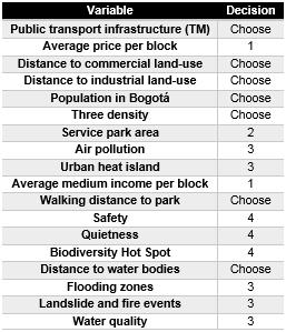
Table 1: Variables that were considered at the beginning for the development of the UGGI

Once the explanatory variables were identified and chose, an OLS model was used to evaluate the linear relationship between the six independent variables with the dependable variable, in order to obtain a global model of the variable. These same steps have been performed in previous research (Anderson, et al., 2014). It was found that the equation that described the regression model is:

Equation 1. OLS regression model representation

Where y correspond to the GS per capita, over time; 𝛽₀ correspond to the intercept of the model, 𝛽₁ till 𝛽_𝑛 represent the coefficient of each independent variables, same as, 𝑋₁ till 𝑋𝑛 which are the value of the explanatory variable; meanwhile the 𝜀 correspond to the residuals of the whole model.

This method assumes linearity in the model and the constant variant. However, spatial data do not always fulfil all the presuppositions that this method of regression requires (He, Okada, Zhang, Shi, & Li, 2008) & (He, Zhang, Shi, Okada, & Zhang, 2006). 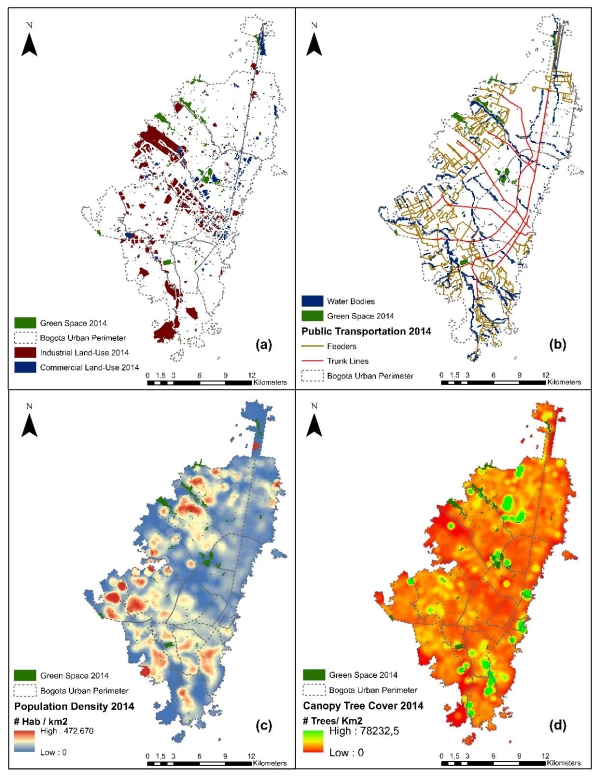In any case, if this method is executed in conjunction with spatial autocorrelation, it could determine if the variables are statistically significant and the model is well specified and has been implemented properly. The Figure 1 and Figure 2 correspond to the spatial distribution of the six explanatory variables chosen for 2005 and 2014.

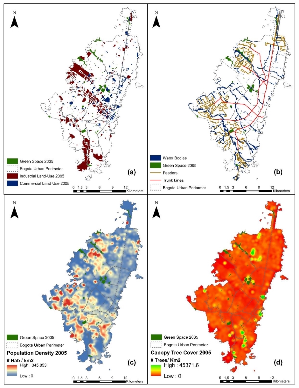
(a): Commercial and Industrial Land-use (b): Public transportation network (c): Population Density (d): Canopy tree cover

Figure 1. Spatial distribution of the population density, canopy tree density cover, public transportation network, water bodies, urban green space, commercial and industrial land uses in Bogotá in 2005, 2014 and 2040

(a): Commercial and Industrial Land-use (b): Public transportation network (c): Population Density (d): Canopy tree cover

Figure 2. (Figure 1 continuation)

Finally, to be able to evaluate the interactions at the spatial level, a Geographic Weighted Regression method was used. This method allows evaluating spatial correlations between neighbouring cells, increasing the specificity of the model and makes it more reliable, as (Yang, Lu, Cherry, Liu, & Li, 2017) assures base on their experience modelling the relationship between active mode travel demands and ambient built-environment attributes; in which they checked that GWR has higher prediction power and provides a more understanding of the spatial variations in the relationships at local and global level. The GWR can be represented by Equation 2:

Equation 2. GWR regression model representation

Where 𝑦𝑖 correspond to the GS per capita or dependable variable, over time; 𝛽0(𝑢0𝑣0) correspond to the intercept of the model with spatial coordinates, 𝛽𝑛(𝑢𝑛𝑣𝑛) represent the coefficient of each independent variables in which values denotes the spatial coordinates for each observation, same as, 𝑋𝑖 till 𝑋𝑛 which is the dimensional vector of K independent variable over time; meanwhile the 𝜀 correspond to the disturbance of the independent and identical distribution.

4. RESULTS

It is imperative to understand that significant changes occurred for a period of only 10 years (Figure 2 and Figure 4) which could suggest that within the results there will be interesting changes and variations. An evaluation of the six selected variables, see Table 1, for 2005 and 2014 were carried out. Firstly, these variables were analysed to determine the relationship with GS per capita. With each of these variables, an exploratory regression analysis was executed. These consisted of a global combination of all variables and with it obtaining the most suitable and descriptive model. Each of the six variables had to meet the following criteria:

1. Probability and Robust Probability (P-Value): Indicates a coefficient is statistically significant (P<0.05).
2. Variance Inflation Factor (VIF): Large values (VIF >7.5) indicates redundancy among explanatory variables.
3. R-squared and Akaike’s Information criteria (IACc): Measures of model fit/performance.
4. Join F and Wald Statistics: Indicates overall model significance (p<0.05)
5.  Koener (BP) statistic: When this test is statistically significant (p<0.05) the relationship modelled are not consistent.
6.  Jarque-Bera Statistic: When this test is statistically significant (p > 0.05) the residuals are not normally distributed.

In addition, it was observed that only four of the six variables in Table 1 were significant in the spatial regression model. Afterwards, an OLS regression model was run with the most representative variables in a global model. Results can be observed in Table 2 and Table 3. In these, the only variable that is representative and can describe the GS per capita in 2005 is population density; meanwhile, in 2014, it was added the coverage of the public transport network as another representative variable. This representability is mainly given by the p-value statistics, even if the rest of the criteria was fulfilled. Likewise, it is important to note that once the p-value is fulfilled, the t-statistics will also be met.

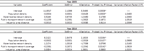
Table 2. Estimate OLS results for the representative variables from 2005 & 2014

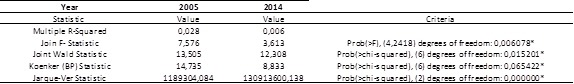
Table 3. Summary of descriptive statistics for the OLS regression model

Once the results of the model have been obtained, it is observed that at present there are only two variables that can explain the GS per capita; of all the possible ones suggested by the literature.

This result suggests that Bogotá is a city that not only lacks green areas for the benefit of its inhabitants but, there is no pattern in the spatial distribution of these zones or enough variables to explain it, something commonly found in cities in developing countries. However, within the research, this was seen as an opportunity to construct a scenario that allowed to explain the spatial distribution of the GS and to quantify it at the level of cell resolution. That is why a much greener scenario for the year 2040 was run; however, to avoid changing any parameter in the “BoLD” model, a new run was decided in which only the zoning will change based on the decree 06 of 1990, of the government of Bogotá, in which establish on the articles 138 and 139 that in the border of the river or the riparian zone of the river must be a protection zone with more than 300 linear meters each side.

Figure 3 shows the modification in the zoning and the land-use map for this new scenario. Figure 4 shows the new green zones, obtained after processing the land-use map for 2040, together with the six variables analysed for the previous years, all following the same procedure described in the methods, with the exception of the canopy tree cover.

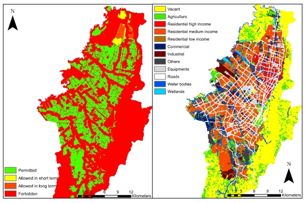
Figure 3. The new zoning and land-use map obtained for this greener scenario in 2040

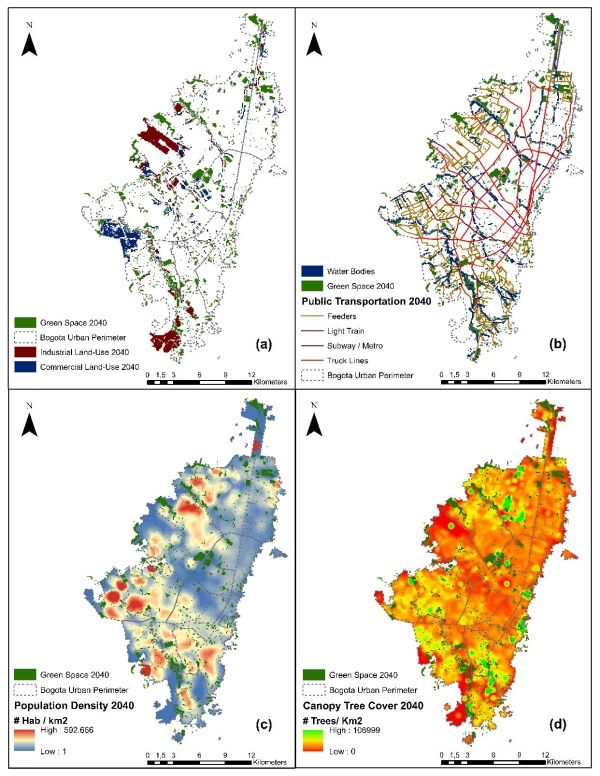
(a): Commercial and Industrial Land-use (b): Public transportation network (c): Population Density (d): Canopy tree cover

Figure 4. (Figure 1 continuation)

For this last variable the procedure that was carried out was the following:

1. Under the international literature, several cities aim to reach an index of 0.30 - 0.50 canopy tree density per inhabitant (MIT, 2017)
2. For the present study, it was considered that in 2040 Bogotá would be at 0.25.
3. By 2014 Bogota had 1,253,533 trees; considering the previous indicator, in 2040 this would rise to 2,549,055 trees.
4. However, growth would not be uniform. In 2014, 28 was the average number of trees per square
   Page 12 of 17 km; so in the future it was decided that all zones above these value will represent 50% of the additional trees; meanwhile, all the zones below the average, that it's almost all the city, will be
   the other half of the increase.
5. So with this method, the average number of trees per km2 would be 57 by 2040, as opposed to a
   uniform extrapolation with an average of only 39 trees per km2. For this scenery, an OLS regression model was run tested again in which the expected result was a significant improvement compared to previous years. The model was once again run with the previous six variables. Once run it, four of the six variables met all the criteria. Although it was a greener scenario, two variables were unable to explain the location and distribution of the GS per capita; they were: canopy tree coverture and the commercial distance measured from the residential land use. In Table 4 and Table 5 it is presented the general diagnosis of the OLS model with main four representative variables.

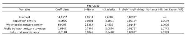
Table 4. Estimate OLS results for the representative variables for 2040

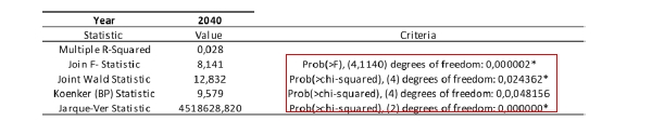
Table 5. Descriptive statistics for the OLS regression model in 2040

With the results obtained within the OLS regression model, it is observed that the global model meets statistical significant. In the local model, the variables will be evaluated at a cell resolution of 100m x 100m of residential land use. The results of the GWR regression model  can be seen in Table 6 for each of the evaluated years. All the models were evaluated with the four significant variables, in which it was observed that at the local level the chosen variables have a greater significance. 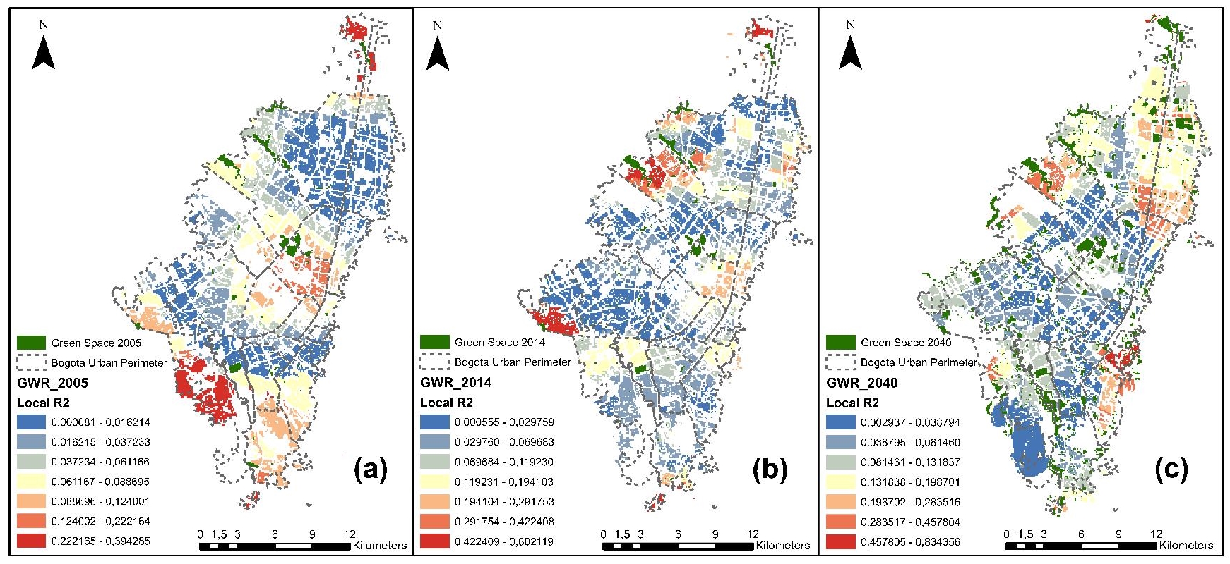Since the  performance in the greener scenario, the spatial pattern of these variables explains more than the 47% of the GS per capita for the year 2040, as can be seen in Figure 5 where the spatial distribution for the local R2 of the model is shown over the time.

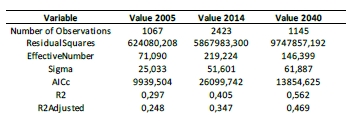
Table 6. GWR result for the three periods of time

Figure 5. GWR Spatial distribution for the local R2 for the UGGI per Capita the three periods of study (click for larger size).

The significance of the model at global and local level, allows to conclude that in the variables evaluated to quantify and measure GS per capita, coincide with those observed in the literature; in turn, it is observed that all the criteria for evaluating an indicator are met, since they are measurable and quantifiable over time. It should be noted that in the current context only two of the four variables can explain the distribution of the current GS; however, under a scenario where the normativity to protect ecosystems and UGS is enforced, the dynamics can change. This is reflected in the fact that in a much greener scenario, all the selected variables are statistically significant and explain in a considerable way the spatial distribution of the green areas; which allows to infer, that under the equations above, these variables can establish at any resolution how much GS per capita there will be in every residential cell in the future.

5. DISCUSSION

In Bogota since 2005, a master plan for the effective public space was established, in which goals were set for 2019. These goals stipulated that by 2015 Bogotá would have a per-capita public space of 6 m2. Today this value is only 4.10 m2. In turn, the same plan stipulated that there would be continuous monitoring and updating of information on indices and GS, as well as increasing and improving afforestation and connectivity rates of urban ecosystems. All of the above would be done with a view to protecting, preserving and guaranteeing the enjoyment of these ecosystems for the community. However, Bogotá currently lacks effective GS at the physical level, and there is no political interest that generates clarity and continuity in this type of policy.

In this master plan of public space, there was no distinction made between private, public, road medians and future GS. Also, it is not clear in how must be interpreted the riparian zones near water bodies. All of the above, generate a challenge in Bogotá when measure GS comes forward; since the benefit and quantification for each of these spaces is different from each other and should not be quantifiable as a whole. Furthermore, the lack of up-to-date information, clear GS plans and up-to-date information generates limitations within the micro-level model.

This limitation occurs when running statistical models since the lack of reliable and updated information will generate more uncertainty within the model. Each variable considered has a unique temporal change and spatial pattern. This implies that for each variable the past and current state was known; however, it was necessary to make an estimate, which is fundamental for land use change models and for decision makers. In the case of transport infrastructure, it should be considered that when looking at the area of influence of a transport network is not done for the entire network but, specifically for the access points, since they are in these where important changes occur; Likewise, for the case of the variable of population density, it must be based on the fact that the last official census that was carried out was in the year 2005. This implies that the spatial distribution of the population could present considerable changes compared to the year 2014, which would imply an important bias for the distribution that would be presented in the year 2040; however, not considering this variable had omitted the most representative and most important variable to measure the GS index in the city. Also, it is important to remember that the other variables that explain the model are mainly a product of the future land policies and territorial planning, which can be changed and present over time.

Although the estimation of each of these variables may present some weakness, calculating and predicting them are fundamental to validate and simulate changes in a LUCC. The predictive models are based on linear and spatial regressions, which allow us to evaluate their representatives over time. In the case of an OLS regression, the representability is determined not only by the p-value but also by the specificity of the variables, which means, that exploratory variables should describe the elasticity of the dependent variable. This indicates the percentage of change of the phenomena due to the independent value (e.g. an increase of population implies a reduction in the GS per capita. Therefore the coefficient that is the numerical value of the change must be negative), as shown in tables Table 2 and Table 4. Also, it is important to always consider the standard deviation and the residual errors as measurements of the quality of the model. In the end, these indicate that the variables are consistent and the model is correct.

GWR model allows evaluating the statistical and spatial impact of one variable over another in a local context, or cell size. This tool allows finding patterns such as areas where there is a greater correlation, compared to areas where deviation and representability are negative. This is a new way of analyzing and understanding the reasons why these zones present this disjunction when explaining the phenomena. In the case of the present study, if a Hot - Cold Spot analysis was made, it would be observed that the areas with the lowest density of GS are those with the lowest R² and lowest statistical representability, which generates a negative impact when evaluating the model in a global way. In the opposite case, when this raster analysis presents a high square R², it shows how explanatory the local model is and how there are incidence and correlation between variables and model in general. Finally, the sum of this allows bringing a global model to a local context, which can change due to the resolution of the model and the information available.

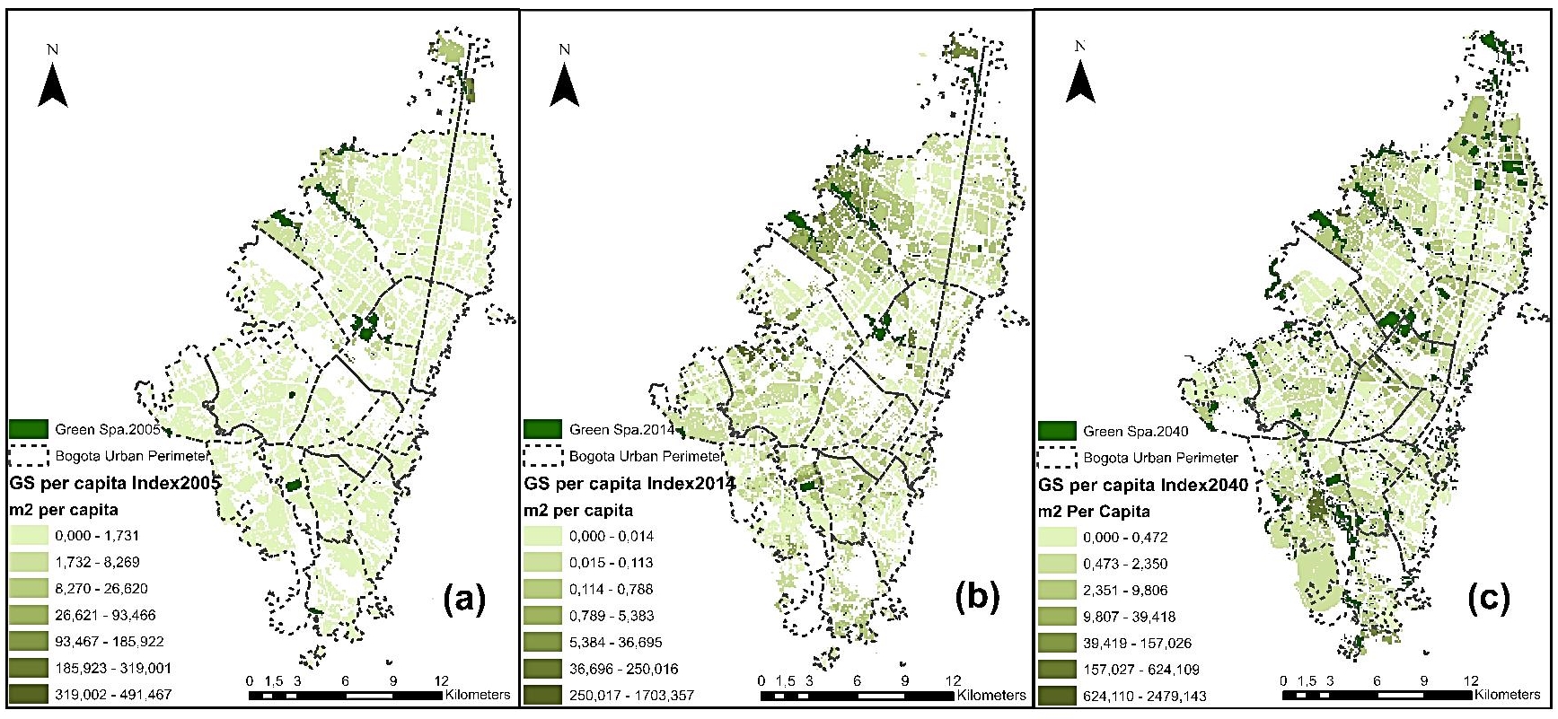
Finally, the proposed scenario for 2040 showed that preserving of the riparian zone, not only a greater GS was obtained, but the intervention in the built area of the city was minimum. Also, considering the population growth, not only an overall increase of the GS was achieved, but in turn, it was observed that the standards of GS per capita in urban Bogotá was above of the suggested by the WHO. It is important to note that even when the “Bold” model includes seven neighbouring municipalities, these were not considered due to the lack of available information. The increase of green areas at the global level and the index of GS per capita for each cell are observed in Table 7 and Figure 6, respectively.

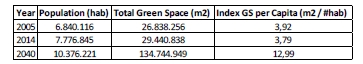
Table 7. Global GS per capita for Bogotá

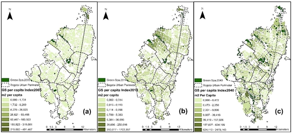
Figure 6 Change in UGS per capita over timey (click for larger size).

6. CONCLUSIONS

The lack of GS in the past and present in the city of Bogotá shows a problem that can still be reversed through clear and concrete actions. Among these actions, it is crucial that the future city plan has a more sustainable approach. That why the LUCC models are used, as it allows to establish greener scenarios with the current city policy. Likewise, the application of Local (GWR) and Global (OLS) regression models allows proposing a methodology to quantify and measure the future GS per capita, through present variables that are quantifiable and can be measured over time. This methodology it is proposed as a way to measure GS in CA models.

Within the research, it was taken into account not only the international literature but also the national and case studies in Bogotá; however, GS in Latin America and in, the Colombian case, are very low; as this is not yet a priority for governments. It is also important to highlight that there are variables that could be much more representative, however such as housing price, crime rate, sustainable projects, land value, urban biodiversity and more; but the lack of updated and detailed information as well as the level of resolution represent an important challenge when estimating future scenarios.

Finally, further research must be done in order to quantify the GS in an integral way, since in compact cities the limiting of land is in conflict with the preservation of ecosystems. That is why, in the long term within these green areas should be counted new urban infrastructures as green roofs, new urban developments and tree canopy density as new GS, which can improve the quality of life of its inhabitants and make cities much more green in an unconventional way.

7. ACKNOWLEDGMENTS

I would like to thank the guidance provided by Professor Daniel Paez and the Group Sur. In turn, thank Professor Abbas Rajabifard and the entire CSDILA team for all the technical support and literature suggested for this research. Any opinions, findings and conclusions expressed in this paper are those of the author and do not necessarily reflect the views of the two research centres.

8. REFERENCES

Alcaldía de Medellín. (2011). BIO 2030 Plan Director Medellín, Valle de Aburrá. Medellín: RMESA. Retrieved from http://www.eafit.edu.co/centros/urbam/Documents/BOOKbio2030plandirectormedellin.pdf

Anderson, W., Guikema, S., Zaitchik, B., Pan, W., Pfeffermann, D., Clayton, D., & Emerson, R. (2014). Methods for Estimating population density in Data-Limited areas: Evaluating Regression and Tree-Based Models in Peru. PLos ONE. doi:10.1371/journal.pone.0100037

Anguluri, R., & Narayanam, P. (2017). Role of green space in urban planning: Outlook towards smart cities. Urban Forestry & Urban Greening, 25, 58 - 65.

Attwell, K. (2000). Urban land resource and urban planting - case studies from Denmark. Landscape Urban Planning, 145 - 163.

Ayuntamiento de Barcelona. (2011). Barcelona green infrastructure and biodiversity plan 2020. Barcelona: Hbitaturba. Retrieved from file:///C:/Users/ja.franco953/Downloads/BCN2020_GreenInfraestructureBiodiversityPlan.pdf

Barbosa, O., Tratalos, J. A., Armsworth, P. R., Davies, R. G., Fuller, R. A., Johnson, P., & Gaston, K. J. (2007). Who benefits from access to green space? A case study from Sheffield, UK. Landscape and Urban Planning, 187 - 195.

Bibri, S. E., & Krogstie, J. (2017). Smart, sustainable cities of the future: An extensive interdisciplinary literature review. Sustainable Cities and Society, 31, 183-212.

Bocarejo, J. P., Portilla, I., & Pardo, M. A. (2013). Impact of Transmilenio on density, land use, and land value in Bogotá. Research in Transportation Economics, 78-86.

Bolund, P., & Hunhammar, S. (1999). Ecosystem services in urban areas. Ecol. Econ., 29, 293 - 301.

Bottalico, F., Chirici, G., Giannetti, F., De Marco, A., Nocentini, S., Paoletti, E., . . . Travaglini, D. (2016). Air pollution removal by green infraestructures and urban forests in the city of Florence. Agriculture and Agricultural Science Procedia, 8, 243 - 251.

Castillo, G. (18 de December de 2013). Indicadores Ambientales de espacio público en Bogotá. Barcelona: Universitat politécnica de catalunya. Obtenido de http://upcommons.upc.edu/bitstream/handle/2099.1/20822/Mem%C3%B2ria%20-%20Ginna%20Alexandra%20CASTILLO.pdf?sequence=1

Connop, S., Vandergert, P., Eisenberg, B., Collier, M. J., Nash, C., CLough, J., & Newport, D. (2016). Renaturing cities using a regionally-focused biodiversity-led multifunctional beneftis approach to urban green infraestructure. Environmental Sicence & Policy. doi:10.1016/j.envsci.2016.01.013

de la Barrera, F., Reyes-Paecke, S., & Banzhaf, E. (2016). Indicators for green spaces in contrasting urban settings. Ecological Indicators, 62, 212 - 219. doi:10.1016/j.ecolind.2015.10.027

Demuzere, M., Orru, K., Heidrich, O., Olazabal, E., Geneletti, D., Orru, H., . . . Faehnle, M. (2014). Mitigatin and adapting to climate change: Multi-functional and multi-scale assessment of green urban infraestructure. Journal of Environmental Management, 146, 107 - 115.

Duh, J. D., Shandas, V., Chang, H., & George, L. A. (2008). Rates of urbanisation and the resiliency of air and water quality. Science of the Total Environment, 400, 238 - 256.

Fan, P., Xu, L., Yue, W., & Chen, J. (2016). Accessibility of public urban green space in an urban periphery: The case of Shangai. Landscape and Urban Planning. doi:10.1016/j.landurbplan.2016.11.007

Force, U. G. (2002). Better Places–Final report of the Urban Green Spaces Task Force. London: Green Spaces. Obtenido de http://www.ocs.polito.it/biblioteca/verde/taskforce/gspaces_.pdf

Gedge, D. (2015, 10 26). 1 European Urban Green Infrastructure conference 2015. Retrieved from Urban Green Infrastructure: http://urbangreeninfrastructure.org/green-tramways-transport/

Gupta, K., Kumar, P., Pathan, S. K., & Sharma, K. P. (2012). Urban Neighborhood Green Index - A measure of Green spaces in urban areas. Landscape and Urban Planning, 105, 325 - 335. doi:10.1016/j.landurbplan.2012.01.003

Gupta, K., Roy, A., Luthra, K., Maithani, S., & Mahavir. (2016). GIS-based analysis for assessing the accessibility at hierarchical levels of urban green spaces. Urban Forestry & Urban Greening, 18, 198 - 211. doi:10.1016/j.ufug.2016.06.005

He, C., Okada, N., Zhang, Q., Shi, P., & Li, J. (2008). Modelling dynamic urban expansion processes incorporating a potential model with cellular automata. Landscape and Urban Planning, 86, 79 - 91. doi:10.1016/j.landurbplan.2007.12.010

He, C., Zhang, Q., Shi, P., Okada, N., & Zhang, J. (2006). Modeling urban expansion scenarios by coupling cellular automata model and system dynamic model in Beijing, China. Applied Geography, 323 - 345.

He, J., Li, C., Yu, Y., Liu, Y., & Huang, J. (2017). Measuring urban spatial interaction in Wuhan Urban Agglomeration, Central China: A spatially explicit approach. Sustainable Cities and Society, 32, 569 - 583. doi:10.1016/j.scs.2017.04.014

James, P., Magee, L., Scerri, A., & Steger, M. B. (2015). Urban Sustainability in Theory and Practice: Circles of Sustainability. London.

Jim, C. Y. (2004). Green-space preservation and allocation for sustainable greening of compact cities. Cities, 21(4), 311 - 320. doi:10.1016/j.cities.2004.04.004

Jim, C. Y., & Chen, S. S. (2003). Comprehensive greenspace planning based on landscape ecology principles in compact Nanjing city, China. Landscape and Urban Planning, 65, 95 - 116.

Jim, C. Y., & Chen, W. Y. (2006). Impacts of urban environmental elements on residential housing prices in Guangzhou (China). Landscape and Urban Planning, 78, 422 - 434.

Jo, H. K. (2002). Impacts of urban greenspace on offsetting carbon emissions for middle Korea. Journal of Environment, 65, 95 - 116.

MIT. (2017). Treepedia: Exploring the Green Canopy in cities around the world. Boston: MIT. Obtenido de http://senseable.mit.edu/treepedia

Natural England. (2010). "Nature Nearby" - Accessible Natural Greenspace Guidance. London: Natural England. Obtenido de www.naturalengland.org.uk/docunents/other/nature_nearby.pdf

New Yorkers for Parks. (2010). The Open Space Index. New York: New Yorkers for Parks. Obtenido de http://www.ny4p.org/research/osi/LES.pdf

Norton, B. A., Coutts, A. M., Livesley, S. J., Harris, R. J., Hunter, A. M., & Williams, N. S. (2015). Planning for cooler cities: A framework to prioritise green infrastructure to mitigate high temperatures in urban landscapes. Landscape and Urban Planning, 134, 127 - 138.

Paez, D. E., & Escobar, F. (2016). Urban transportation scenarios in a LUCC model: a case study in Bogota, Colombia. Bogotá.

Pakzad, P., & Osmond, P. (2016). Developing a sustainability indicator set for measuring green infrastructure performance. Social and Behavioral Sciences, 68 - 79.

Pauleit, S., & Duhme, F. (2000). Assessing the environmental performance of land cover types for urban planning. Landscape Urban Planning, 52, 1 - 20.

Scopellieti, M., Carrus, G., Adinolfi, C., Suarez, G., Colangelo, G., Lafortezza, R., . . . Sanesi, G. (2016). Staying in touch with nature and well-being in different income groups: The experience of urban parks in Bogotá. Landscape and Urban Planning, 148, 139 - 148.

Tzoulas, K., Korpela, K., Venn, S., Yli-Pelkonen, V., Kazmierczak, A., Niemela, J., & James, P. (2007). Promoting ecosystem and Human health in urban areas using Green Infrastructure: A literature review. Landscape and Urban Planning, 81, 167 - 178.

WHO. (s.f.). Urban Green Spaces and Health: A review of the evidence. WHO Regional Office for Europe. Copenhagen: WHO. Obtenido de http://www.euro.who.int/__data/assets/pdf_file/0005/321971/Urban-green-spaces-and-health-review-evidence.pdf?ua=1

Wolch, J. R., Byrne, J., & Newell, J. P. (2014). Urban green space public health, and Environmental Justice: The challenge of making cities "Just green enough". Landscape and Urban Planning, 125, 234 - 244. doi:10.1016/j.landurbplan.2014.01.017

Wu, J. (2014). Urban ecology and sustainability: The state of the science and future directions. Landscape and Urban Planning, 209-221.

Yang, H., Lu, X., Cherry, C., Liu, X., & Li, Y. (2017). Spatial variations in active mode trip volume at intersections: a local analysis using geographically weighted regression. Journal of Transport Geography, 64, 184 - 194. doi:10.1016/j.jtrangeo.2017.09.007

Yin, X., Olesen, J. E., Wang, M., Ozturk, I., & Zhang, H. (2016). Impacts and Adaptation of the cropping systems to climate change in the northeast Farming Region of China. European Journal of Agronomy, 78, 60-72.

Zeng, C., Zhang, M., Cui, J., & He, S. (2015). Monitoring and modelling urban expansion - A spatially explicit and multi-scale perspective. Cities, 92-103. doi:10.1016/j.cities.2014.11.009

Zuccalà, M., & Verga, E. S. (2017). Enabling energy smart cities through urban sharing ecosystems. Energy Procedia, 826 - 835.