Article of the Month -
February 2011
|
Validation of the Laboratory Calibration of Geodetic
Antennas based on GPS Measurements
Philipp ZEIMETZ and Heiner KUHLMANN, Germany


 This article in .pdf-format
(16 pages, 455 KB)
This article in .pdf-format
(16 pages, 455 KB)
1) This paper is a peer reviewed
paper presented at the FIG Congress in Sydney, Australia in April 2010.
The topic of the paper is relevant to all who are interested in high
precision GNSS surveying and it is presenting a new and innovative
method for antenna calibration.
Key words: GNSS antenna calibration, GPS, calibration
accuracy, anechoic chamber, laboratory calibration, near-field
SUMMARY
In relative GNSS positioning, the antenna effects are one of the
accuracy limiting factors. Besides relative and absolute field
calibration procedures, there is an absolute laboratory calibration
procedure, which is used at the University of Bonn. Since February 2009
a new antenna calibration lab, which is especially concepted for the
antenna calibration, is operable.
This paper presents some investigations on the accuracy of this
calibration procedure. The results are mainly based on GPS height
measurements and the comparison with the results from a precise
levelling. For this purpose 121 baselines between the 8 pillars of an
EDM calibration baseline site with distances between 18 and 1101 meters
were analysed. The levelled height differences can be regarded as
references, thus it is possible to quantify the absolute GPS-accuracy.
Furthermore, the GPS-accuracy is an indicator for the antenna
calibration accuracy.
The measured height differences are usually smaller than 1-2 mm
(maximal deviations), when using the L1 or the L2 frequency, thereby the
standard deviation is 0.8mm in both cases. As expected, in case of the
ionospheric free linear combination L0 the standard deviation rises up
to 3 mm. This very high accuracy is possible if besides other effects,
the antenna effects are reduced to a minimum level (e.g. the differences
between an individual calibration and a type calibration can reach
several mm). It is not possible to quantify the accuracy exactly,
because the antenna effect is only one of various remaining
uncertainties. Thus, the effects due to the calibration uncertainties
are smaller than s = 0.8mm, at least.
This high accuracy cannot be reached if dominant near-field effects
exist. Near-field effects, which cannot be separated from the behaviour
of the antenna itself, limit the accuracy of the relative GPS. Such
effects are present in some of the analysed baselines, too. Here, one
special antenna-near-field combination causes height differences of
several millimeters. The other GPS results show an exceedingly high
accuracy and give an idea of the high calibration accuracy.
1. INTRODUCTION
The phase center of the receiver antenna is the reference point where
each GPS/GNSS observation (phase measurement) refers to. Since the phase
measurement and, as a consequence, the determined signal path length
between antenna and satellite depend on azimuth a and elevation b of the
incoming signal, the antenna is not a point in mathematical sense. The
purpose of the antenna calibration is to determine the deviations from
an ideal point-like antenna as a function of the direction of the
incoming signal (see e.g. Geiger 1988).
Since the 1980’s different calibration procedures have been
developed. Beside the relative and the absolute field procedures, an
absolute laboratory calibration procedure exists. This procedure, which
is ideally performed in anechoic chambers, is a standard technique in
radio-frequency engineering (e.g. Kraus and Marhefka 2003). Such a
laboratory procedure was developed at the University of Bonn and a new
anechoic chamber is operable since February 2009. The realisation of the
calibration laboratory is a cooperation between the University and the
Bezirksregierung Köln (District Government of Cologne).
The accuracy of the calibration results has been assessed by
comparisons with the field procedures in earlier works (Zeimetz and
Kuhlmann 2006 or Zeimetz et al. 2009). Additionally, the calibration
results can be analysed by applying them for GPS-measurements. To avoid
that other GPS uncertainties dominate the antenna effects, it is useful
to make these tests in a small local GPS network. For this purpose an
Electronic Distance Measurement (EDM) calibration baseline site of the
Bundeswehr (German Federal Armed Forces) could be used. The differences
between the GPS solutions and the precise levelling visualize in the
first place the GPS accuracy and thus among others the remaining antenna
effects.
A remaining problem is the near-field problem. The near-field depends
primarily on the mounting of the antenna (pillar/tripod, tribrach,
spacer). Differences between the setup in case of calibration and in
case of GPS-measurement can be reduced but not eliminated. The
near-field affects mainly the height component, as it becomes visible in
the tests presented here.
2. ANTENNA PROPERTIES
The GNSS receiver antenna converts the electromagnetic satellite
signals into electrical currents. After the conversion of the signal,
the remaining path length (cable, electronic components) is similar for
all satellite signals (except for small amounts), thus, the estimated
GPS-position refers to the antenna or more exactly to the so called
phase center. This view is only correct if the phase measurements would
always refer to one fixed point. In reality, the measured phase depends
on the direction (azimuth a and elevation b) of the incoming signal,
thus, the so called phase center variations (PCV), which describe the
deviations from a mean phase center, have to be considered. The position
of the mean phase centre with respect to the antenna reference point
(ARP) is usually described by the phase center offset. This
classification of PCO and PCV can be found in earlier works on this
topic (e.g. Geiger 1988). The corresponding antenna model is illustrated
in Fig. 1.
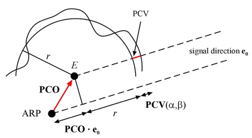
Fig. 1: Antenna model (Zeimetz and Kuhlmann 2008).
The measured range sARP (resp.
phase) depends on the direction of the incoming signal:

with r being the error-free value, e0
the unit-vector in the direction
a and
b of the
satellite and
e
the noise of the observations. A separation of the effects of PCO and
PCV is not possible, because for every position of E, a specific set of
PCV exist which describe the antenna correctly. In order to solve the
singularity the condition
can be used.
Because the PCV can reach values up to 20 mm it is
always necessary to use the full antenna model (not only the PCO) if
highest accuracy is required. Examples of the phase center variations
are presented e.g. in Zeimetz and Kuhlmann 2006.
3. ANTENNA CALIBRATION IN THE ANECHOIC CHAMBER BONN
The main idea of the laboratory antenna calibration procedure is to
simulate the different signal directions by rotations of the
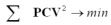
GNSS-antenna (Schupler et al. 1994). Therefore, the calibration setup
consists of a fixed transmitter on the one end and a remote-controlled
positioner carrying the test antenna on the other end of the test range
(Fig. 2). At every selected antenna position (equal to a satellite
direction) a network analyser (NWA, here Agilent ENA E5062A) generates a
signal which is transmitted in the direction of the GNSS antenna. The
GNSS antenna is also connected with the NWA, thus, the NWA can measure
the phase shift between the outgoing and incoming signals. This phase
delay depends on the signal direction. Since the outgoing signal is
constant, a grid of phase corrections is directly obtained as a result
of the calibration. Usually a frequency range from 1.15 to 1.65 GHz is
used, whereby only the frequencies of GPS, GLONASS and GALILEO are
usually analysed.
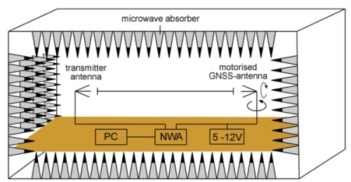
Fig. 2: Setup of the anechoic calibration facility
(Zeimetz and Kuhlmann 2008).
Regarding GPS, multipath and near-field effects are one of the
largest sources of error (e.g. Wanninger and May 2000). In case of
calibration the multipath effects can be reduced to a low level by using
special anechoic chambers (Fig. 3), whereas the near-field problems
cannot be avoided. As in case of normal GPS applications, the nearby
environment of the antenna has an influence on the electromagnetic field
and thus on the phase measurement.
Fig. 3: Antenna calibration laboratory Bonn (without antenna positioner)
4. POSSIBILITIES FOR THE VALIDATION OF THE CALIBRATION ACCURACY
The quality (accuracy and precision) of a measurement system can be
quantified if there is an alternative procedure with a significantly
higher accuracy (factor 3 or more). In case of antenna calibration there
are independent calibration systems, but no one which is suitable as
reference. Nevertheless, there are possibilities to quantify the
accuracy. The different methods for the analysis of the calibration
results can be divided into two classes:
- Analyses by comparison of calibration results on the level of
different phase patterns.
- Determining the accuracy of the calibration by GPS-measurements
in GPS test sites.
Comparison of phase patterns
In order to determine the calibration accuracy, it is possible to
compare the results from different independent calibration procedures
(comparisons between laboratory-, relative- and absolute field
calibration). This approach supplies a very clear look at the
differences between two patterns, but there are two important
disadvantages. (1) Only the agreement between two different antenna
patterns can be tested. It is not possible to distinguish the
differences between the compared antenna patterns into two parts. An
absolute accuracy cannot be determined. (2) The effect of the
calibration uncertainties on the GPS-measurements cannot be derived from
such comparisons. Analysis on the accuracy of the laboratory calibration
procedure of the university of Bonn, which are based on direct
comparisons of different procedures, were published e.g. by Zeimetz
and Kuhlmann 2006 or Zeimetz et al. 2009.
Determining the calibration accuracy by GPS-measurements
To determine the accuracy of calibration by measurements at a test site,
a reference solution is necessary. But, instead of being dependent on
GPS, other systems (EDM, precise levelling) can be used as reference.
The disadvantage is, that the estimated GPS accuracy is not equal to the
calibration accuracy, because of additional uncertainties (e.g.
multipath, near-field, tropos-phere). But it becomes obvious, which GPS
accuracy can be achieved, when using these calibration patterns and
especially when different antenna types are combined. Then, in some
cases, the effects of multipath or near-field variations can be
quantified, what leads to a more precise statement about the calibration
accuracy (as in case of the near-field, chapter 5).
4.1 Testing the antenna calibration on an EDM calibration baseline
It is obvious that antenna calibration results can be tested by GNSS
measurements. Due to the large number of other measurement uncertainties
such as troposphere effects, multipath, near-field effects and of course
random deviations, it is necessary to get a sufficient sample size. A
large test campaign was carried out in June 2009. Beside a large sample
size of altogether 122 baselines, different setups have been chosen in
order to consider the following aspects:
- same antenna, same mounting, different location (to ensure that
multipath effects would not be interpreted as antenna effects)
- same antenna, different mounting, same station (to test the
near-field effect)
- different antennas (to see the antenna effect)
As relative GPS is used, it is necessary to have a look at both
involved setups.
The following 9 antennas with individual calibrations were used (3
different antenna types):
- 3 LEIAT504GG (Leica AT504GG Choke Ring Antenna)
- 3 TRM41249.00 (Trimble Zephyr Geodetic)
- 3 TRM55971.00 (Trimble Zephyr Geodetic 2)
Because of the high degree of effort only three antenna types could
be considered until now. Perhaps it is possible to complement these
antennas, which are most prevalent in GPS networks, by further tests in
the future.
The EDM calibration baseline site antenna mounting
The EDM calibration baseline site (facility of the University of the
German Federal Armed Forces) consists of 8 pillars. The distances
between the 8 pillars vary from 18 to 1101 meters. The height
differences between the top of all pillars are less then 30 mm. Each of
the pillars has a height of approximately 1.6 m and all pillars are of
the same type, whereas for the mounting of the antenna two different
setups were used (see Fig. 4).
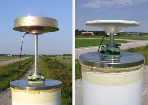
Fig. 4: Pillars and antenna mounting
The conditions are very good for precise GNSS-Measurements. The
pillars are placed on an earth mound, thus the top of the pillars are
between 3 and 4 meters above the surrounding surface level. The fence,
visible on the left photo, should produce only short-periodic multipath
effects because of the large (vertical and horizontal) distance between
the fence and the antennas (e.g. Bilich et al. 2007). In case of such
short-periodic multipath effects and an observation time of several
hours, only weak multipath effects are expected. As the surface of the
mound is uneven and not hard-surfaced, the mound itself should also
produce only weak multipath signals.
Significant ionospheric and tropospheric effects on the GPS results
could not be excluded, even in case of short baselines (e.g. Santerre
1991). However, these effects should be very small and depend on the
distance between the pillars, thus, these effects would become visible
as systematic differences (depending on the distance). Anticipating the
analyses, such effects could not be detected, thus, they can be
neglected in the current state of accuracy.
Observation time:
In order to increase the number of different antenna configurations, the
observation time has been reduced to a duration between 4 and 10 hours.
Especially for the determination of the height, longer observation times
are generally used. These observation times were sufficient here, as
shown in chapter 5.
4.2 Terrestrial Reference Measurements
For the validation of the GPS measurements, terrestrial reference
measurements can be used. The pillar heights have been measured by
precise levelling and the distances between the pillars have been
determined by EDM measurements.
4.2.1 EDM
The accuracy of the EDM is limited primarily by atmospheric effects.
Despite the measurement of temperature, pressure and humidity a scale
error of about 1 – 2 ppm has to be expected due to mismodeling the
effect of atmosphere. Considering the accuracy of the EDM (Leica TPS
1201+; 1mm + 1.7ppm) the total accuracy is between 1 and 3 mm depending
on the distance, thus the EDM accuracy is comparable with the GPS
accuracy. As the EDM measurements serve for independent results, they
can be used for the detection of outliers.
4.2.2 Precise levelling
The height differences between neighboured pillars are measured twice
by precise double-levelling. The differences between both solutions are
smaller than 0,2 - 0.3 mm. Only in case of the baseline between pillars
7 and 8 the deviation is larger (0.4 mm). The antenna heights (heights
above the pillars) are measured by levelling, too. Here an accuracy of
0.1 0.2 mm can be assumed.
When comparing GPS and levelling results, it is necessary to become
aware of the different reference levels. The GPS results are related to
the used reference ellipsoid (here: GRS80), whereas the levelling
depends on the local gravity field. Comparing GPS and levelling, the
angle between the ellipsoid normal and the local vertical and the
resulting effect on the height determination has to be considered (Flury
et al. 2009). For the area of the Federal Republic of Germany the
quasigeoid GCG05 (German Combined QuasiGeoid 2005) enables the
conversion between ellipsoidal heights (ETRS89) and normal heights
(DHHN92). The calculated quasigeoid heights increase from 45.610 m
(pillar 8) to 45.636 m (pillar 1). As the normal of the quasigeoid and
the direction of the local gravity field do not coincide, remaining
relevant deviations are possible. Such height differences would increase
with the distance between two pillars (because of the tilt angle between
the surfaces), however, such systematic effects are not visible in the
results (Fig. 6).
5. RESULTS
The campaign consists of 5 sessions. In the first session only 5
pillars could be used, whereas in the other session all 8 pillars were
equipped with GPS antennas. Thus, 32 independent baselines were
observed. Additionally 90 baselines can be created using the same
observations (satellite signals). To have a look at all solutions is
quite meaningful. Thereby the effect of the antennas and especially of
antenna combinations can be analyzed. Correlations between the
observations due to using the same signals are not relevant here. It is
rather an advantage when station independent effects are correlated
(e.g. correlations from atmospheric effects, orbit erros or the
satellite geometry), thus station dependend effects become more
significant.
To get a first impression about the quality of the measurements, the
differences between the precise levelling (geoid corrections are
considered as described above) and the GPS-measurements are visualized
in Fig. 5 (L1, 10° elevation cut-off, without troposphere parameter
estimation), where the sorting of the baselines is random. The maximum
deviations are less than 2 mm and the corresponding standard deviation
is 0.8 mm. The distribution of the results is very similar to the
theoretical Gaussian Distribution (see histogram, Fig. 5).
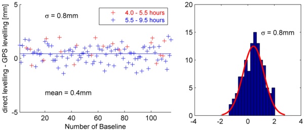
Fig. 5: Differences between GPS and presice leveling
(L1) – sorting: random
The determined offset of 0.4 mm is significant. The
cause is yet unknown, but a few possibilities could be excluded. Fig. 6
shows the same results as Fig. 5, but the sorting is different
(displayed are all baselines < 630 m i.e. more than 90% of the results).
Because there are no effects which depend on the baseline length,
ionospheric effects, tropospheric effects and effects of the different
reference levels (ellipsoid vs. geoid) can be discarded. Antenna effects
are possible, but because of antenna swaps the mean should be zero or at
least not significant.
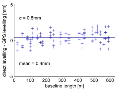
Fig. 6: Differences between GPS and presice leveling
(L1) - sorting: baseline length
Altogether, the L1-GPS solutions are quite good, especially as there
are also uncertainties from the levelling (see chapter 4.2). In case of
relative height determination with GPS, this high accuracy is possible
if besides multipath and near-field effects also the antenna effects can
be reduced to a very low level. This is especially important when
baselines with mixed antennas are analysed, too.
For the sake of completeness, it should be mentioned that the results
of one station (session 5, pillar 8, à 7 baselines) were eliminated. The
deviations are, independent from the choice of the second GPS-point,
five times larger than the calculated standard deviation. Thus, these
solutions are eliminated as outliers. One possible explanation is that
the observation time is very short here (4 hours). However, the fact
that the differences between the L1- and the L2-solutions are only
around 2 mm contradicts this theory. Another possible explanation is
that the antenna height was not measured correctly, but this cannot be
clarified afterwards.
Even, because of these results, it is important to check whether an
increase of time causes a significant higher accuracy. Therefore in Fig.
5 results are displayed in red, when the observation time is between 4
and 5.5 hours. As the distribution of the red samples is very similar to
that of the other results (blue = 5.5 – 10 hours), the observation time
of at least 4 hours is suitable in this case. The standard deviation of
the red samples is 0.8 mm as well.
In the next step the L2-solutions are analysed (Fig. 7). The offset
of 0.5 mm is equal to the "L1-offset" of 0.4 mm in a statistical sense.
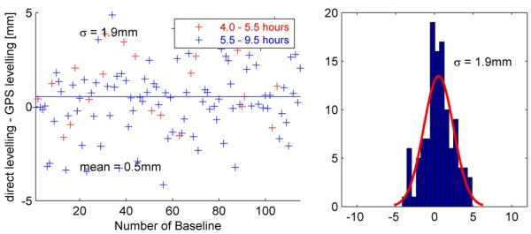
Fig. 7: Differences between GPS and presice leveling
(L2)
More important is that the standard deviation is twice as large as in
case of L1. A lower accuracy for L2 is typical, but the ratio between
sL1 and sL2 is too large. Systematic effects cannot be seen in the
results, but the histogram shows some deviations from the theoretical
form (red line). This is not unusual for GPS-measurements, but regarding
the ionospheric free linear combination L0 these deviations become more
obvious (histogram, Fig. 8). A lot of measurements (57) have a deviation
of only ±1mm in comparison to the levelling. On the one hand the
histogram shows that the calculated value for the standard deviation is
too high for these samples. On the other hand there are too many
deviations which could not be explained by random noise.
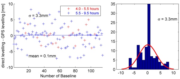
Fig. 8: Differences between GPS and presice leveling
(L0)
Since the L1 solutions do not show such systematic effects, there has
to be an effect, which affects L1 and L2 in a different way.
Impact of the near-field
It is common knowledge that the near-field of the antenna changes the
behaviour of the electromagnetic field of the antenna and as a
consequence the phase measurement of the antenna (see Wübbena et al.
2006). In case of the presented GPS-measurements, 3 antenna types and 2
different setups were used. By combining different antenna types and
different antenna near-fields (mounting) it is here possible to detect
near-field effects and ensure that no other effects (e.g. multipath,
ionosphere) cause the problems which are visible for L2.
In Fig. 9 (left) the differences between GPS and the precise
levelling are visualized in a grid (session2, L2, 10° elevation cut
off). This grid shows the difference between GPS and levelling heights.
In case of the baseline between the pillars 1 and 2 (first box, top,
left) the difference is e.g. 2.2 mm. The exact value is displayed if a
limit of 1.5 mm is exceeded. If the value is smaller, the difference is
depicted only in form of the color coding. This representation was
chosen to highlight the relevant values. Additionally the left axis is
labeled with the corresponding antenna types.
504
= LEIAT504GG = Leica AT504GG (Choke Ring Antenna)
TRM1
= TRM41249.00 = Trimble Zephyr Geodetic (GPS)
TRM2
= TRM55971.00 = Trimble Zephyr Geodetic 2 (GNSS)
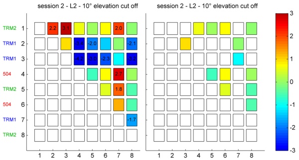
Fig. 9: Differences between GPS and presice leveling
(L2) – Session 2 (right figure without combinations with one TRM1
antenna
Obviously, the largest differences appear if one TRM1 antenna is
involved. In these cases, the signs and the amplitudes of the
differences are similar (regard the direction: Dh12 = - Dh21). The mean
value of these differences is 2.6 mm. When using two TRM1 antennas, the
limit will not be exceeded, because similar systematic effects are
eliminated in case of relative GPS (baselines 2-3, 2-7, 3-7). In the
right figure all combinations with one TRM1 antenna are faded out, what
facilitates the comparisons. All deviations are smaller than 1.5 mm.
In session 4 one major change has been applied w.r.t. session 2, i.e.
the antennas at the pillars 1, 2 and 8 have been equipped with a 255 mm
distance piece (Fig. 4 left). In Fig. 10 this is marked by the vertical
line in the antenna type name (e.g. “TRM1 |”). As a consequence, the
modified TRM1 antenna at point 2 does not show the same (abnormal)
behaviour as the ones at point 4 and 7 (mounted as shown in Fig. 4;
right). The latter ones behave as in session 2 (Fig. 9). Thus, the
changed near field produces a deviation of around 4 mm (Fig. 10; right).
Furthermore, the setup with the distance piece shows a good (better)
agreement with the levelling.
In addition it is obvious that only the TRM1 antennas show such
strong near-field effects. Whereas in case of the Choke Ring antenna
(504) this can be explained by the better shielding, the behaviour of
the TRM2 antenna, which outwardly looks like a TRM1 antenna, was not
expected.
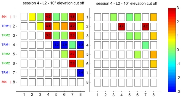
Fig. 10: Differences between GPS and presice leveling
(L2) – Session 4 (right figure without combinations with one TRM1
antenna)
The discussed effects are visible in almost all sessions, however
there are examples where the behaviour is different. In session 5 (Fig.
11) point 4 (TRM1 | without significant effects) and point 7 (TRM1 with
significant effects) behaves as expected. But the result of point 2
(TRM1) clearly deviates from the other ones. In general the results of
session 5 are slightly different. For example, there are comparative
high differences at the baselines 1-3 and 3-5, where TRM2 and 504
antennas were used. In absolute terms the deviations are very small (1.8
and 1.7 mm) and perhaps the results of random uncertainties. Other
reasons for the deviations in comparison to the other sessions are:
- - Rainfall during the session
- - Observation time (session 5 was the shortest one)
- - Changed environments (e.g. changing multipath environment
because of rainfall).
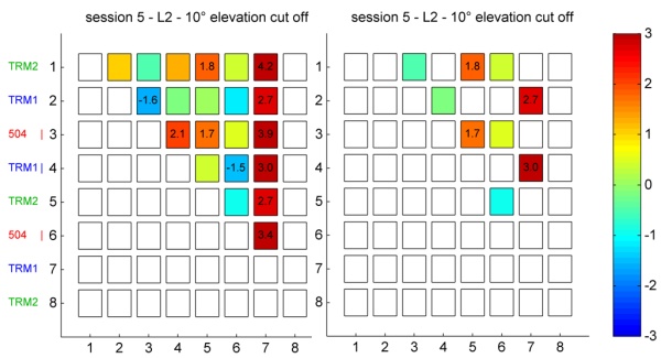
Fig. 11: Differences between GPS and presice leveling
(L2) – Session 5 (right figure without combinations with one TRM1
antenna)
The size of the detected near-field effects becomes clear if the
results of all sessions are visualized in one figure (Fig. 12). The
sorting of the baselines is again random. The baselines where exactly
one TRM1 (without distance piece) antenna was used, are displayed in
red. If two TRM1 were used, the results are colored in green.
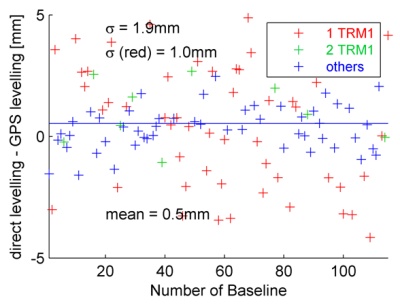
Fig. 12: Differences between GPS and
presice leveling (L2) with highlighted near-field effects
The red samples spread around +2.5 mm and –2.5 mm.
Altogether, the blue and green ones show a better agreement with the
results from the precise levelling. The standard deviation of the
reduced sample (blue & green samples; “TRM1 |” setups are included) is
sL2,red = 1 mm and very similar to the L1 solutions. (sL1= 0.8 mm, see
Fig. 5). Of course the L0 results show the same systematics (Fig. 13).
For the sake of completeness: for the L1 solutions such effects are not
visible as expected because of the results displayed in Fig. 5.
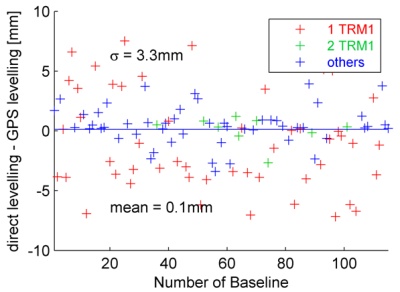
Fig. 13: Differences between GPS and presice leveling
(L0) with highlighted near-field effects
As presented above, the reason for the great deviations in case of L2
is the effect of the near-field, when using the antenna-mounting
combination displayed in Fig. 4 (right). But it is useful to discuss,
whether other effects could play a contributory role, too.
multipath: Improbably because multipath effects are
site-dependent and the here discussed effects are visible for one
special antenna-mounting-combination and not only at special pillars.
antenna calibration: In case of calibration there are
near-field effects as in the case of GPS-measurements. A separation of
the antenna-field and the near-field is not possible as mentioned above.
Other systematic effects of the calibration should be similar for all
antennas, thus the effects are eliminated in case of relative GPS.
atmospheric effects and satellite orbit error: These effects
depend on the baseline length, but they are independent from the
receiver antenna. The visible effects are independent of the baseline
length.
Finally, it has to be noted that in the here presented case a Trimble
Zephyr Geodetic antenna reacts on changes in the near-field. This result
is only valid for the tested antenna-mounting combination. It is
possible that in other environments other antennas react sensitively.
6. CONCLUSIONS AND OUTLOOK
In order to review the validity of the absolute chamber antenna
calibration procedure, GPS-height measurements are compared with the
results of a precise levelling. Based on these measurements, an accuracy
of around sHeight
1 mm could be proven (sL1=0.8
mm and
sL2=1
mm). But it has to be remarked, that in case of one
antenna-mounting-combination larger differences were found. These
differences were caused by the near-field of the antenna and not by
remaining uncertainties of the calibration.
In cases without such strong near-field effects, the remaining
uncertainty budget is composed mainly of multipath, near-field and
tropospheric effects, the remaining uncertainties of the antenna
calibration and of the precise levelling. As shown above, it is of
secondary importance to obtain the exact amount of the calibration, as
long as the near-field problem is not solved. Within the limits of the
determined accuracy, the calibration is valid for at least the three
tested antenna types.
The general benefit of the antenna calibration in absolute terms has
not been discussed in this paper. This has been done in earlier works on
this topic (e.g. Menge 1998). More interesting is how good the
agreement between the currently available calibration procedures is. As
for each of the calibration procedures e.g. the mountings of the
antennas and so the near-field effects are not equal, differences should
become visible if the results of different calibration procedures will
be mixed. It is interesting whether it is possible to mix the procedures
without a reduction of accuracy. This should be answered by further
investigations. The existing data set is well suitable for this task. In
a first step, all 9 antennas have to be calibrated with alternative
procedures (if possible with relative and absolute field procedure).
Hopefully, the analyses with mixed calibrations leads to some new
findings about the calibration accuracy and the near-field problem.
-
Bilich, A., Larson, K. M., 2007, “Mapping the GPS
multipath environment using the signal-to-noise ration (SNR), Radio
Science, Vol. 42, No. 2, CI: RS6003.
-
Flury, J., Gerlach, C., Hirt, C., Schirmer, U, 2009,
“Heights in the Bavarian Alps: mutual validation of GPS, levelling,
gravimetric and astrogeodetic quasigeoids”, Geodetic Reference
Frames, IAG Symposia, Vol. 134, pp. 303-308, Munich.
-
Geiger, A., 1988, „Einfluss und Bestimmung der
Variabilität des Phasenzentrums von GPS-Antennen“, Mitteilungen des
IGP der ETH-Zürich, No. 43, Zurich, Institut für Geodäsie und
Photogrammetrie an der ETH-Zürich.
-
Kraus, J.D., Marhefka, R.J., 2003, “Antennas: for
all Applications”, third edition, McGraw Hill.
Menge, F., 1998, „Zur Kalibrierung der Phasenzentrumsvariationen von
GPS-Antennen für die hochpräzise Positionsbestimmung“, Wiss. Arb. d.
Fachr. Verm., 247, University of Hanover.
Santerre, R., 1991, “Impact of GPS Satellite Sky Distribution”,
manuscripta geodaetica, Vol. 16, pp. 28-53.
-
Schupler, B.R., Allshouse, R.L., Clark, T.A., 1994,
“Signal Characteristics of GPS User Antennas”, Navigation, 41(3),
pp. 277-295, Institute of Navigation.
-
Wanninger, L., May, M., 2000, “Carrier Phase
Multipath Calibration of GPS Reference Stations”, Proceedings of the
13th International Technical Meeting of the Satellite Division of
the Institute of Navigation ION GPS 2000, Salt Lake City, Utah, USA.
-
Wübbena, G., Schmitz, M., Boettcher, G., 2006,
“Near-field Effects on GNSS Sites: Analysis using Absolute Robot
Calibrations and Procedures to Determine Corrections”, Proceedings
of IGS Workshop 2006 “Perspectives and Visions for 2010 and beyond”,
Darmstadt, Germany.
-
Zeimetz, P., Kuhlmann, H., 2006, “Systematic effects
in absolute chamber calibration of GPS antennas”, Geomatica, 60/3,
pp. 267-274, Ottawa, Canadian Institue of Geomatics.
-
Zeimetz, P., Kuhlmann, H., 2008, “On the Accuracy of
Absolute GNSS Antenna Calibration and the Conception of a New
Anechoic Chamber”. Proceedings of the FIG Working Week 2008, 14.-19.
June, Stockholm, Sweden.
-
Zeimetz, P., Kuhlmann, H., Wanninger, L., Frevert,
V., Schön, S., Strauch, K., 2009, Ringversuch 2009, 7.
GNSS-Antennenworkshop, 19.-20. March 2009, Dresden, Germany.
http://tu-dresden.de/die_tu_dresden/fakultaeten/fakultaet_forst_geo_und_hydrowissenschaften
/fachrichtung_geowissenschaften/gi/aws09/7AWS09_07_Zeimetz.pdf
BIOGRAPHICAL NOTES
Mr. Philipp Zeimetz holds a diploma degree in geodesy from the
University of Bonn, Germany. He is a scientific assistant at the
Institute of Geodesy and Geoinformation of the University of Bonn. His
research is mainly focussed on the calibration of GPS-antennas.
Prof. Dr. Heiner Kuhlmann is full professor at the Institute of
Geodesy and Geoinformation of the University of Bonn. He has worked
extensively in engineering surveying, measurement techniques and
calibration of geodetic instruments.
CONTACT
Philipp Zeimetz
University of Bonn
Institute of Geodesy and Geoinformation
Nußallee 17
53115 Bonn
GERMANY
Tel. +49 228 733565
Email: zeimetz@igg.uni-bonn.de
Website: www.gib.uni-bonn.de
 |


