Article of the Month -
October 2013
|
From Passive to Active Control Point Networks – Evaluation of Accuracy
in Static GPS Surveying
Pasi HÄKLI, Ulla KALLIO and Jyrki PUUPPONEN, Finland
1) This peer reviewed paper
was presented at FIG Working Week in Abuja, Nigeria, 8 May 2013 and
evaluates the accuracy of static GPS surveying through active stations
with regard to the official passive control point networks in EUREF-FIN.
Key words: active stations, passive stations,
GNSS, VRS, network-RTK, control point, positioning accuracy
SUMMARY
Over the past decade, active GNSS stations have
become increasingly essential for surveying. Positioning services, such
as network-RTK, have revolutionized surveying practices and challenged
traditional control point networks and the ways of measuring them. A
change from a passive to active definition of control point networks
would require a comprehensive change in measuring principles. Until now,
surveyors making geodetic measurements have been obliged to do the
measurements hierarchically relative to the nearest higher order control
points.
In Finland, the definition of the national ETRS89
realization, EUREF-FIN, is based on traditional passive networks instead
of active GNSS stations. Since the average spacing of active stations in
network-RTK services is approximately 70 km, and for passive networks
much less, the use of active stations would require measurements
neglecting the hierarchy of the (defining) passive networks. In this
paper, we evaluate the accuracy of static GPS surveying through active
stations with regard to the official passive control point networks in
EUREF-FIN.
The results of this study allow us to conclude that
the consistency of static GPS surveying from active GNSS stations with
respect to the official hierarchical passive control point network is in
the order of 1–3 cm (rms). However, some systematic features can be
seen. One issue that needs more careful consideration is the
determination of ETRS89 coordinates for active GNSS networks. In
Finland, the reference frames (i.e. positions of control points) are
influenced by postglacial rebound that challenges the determination and
maintenance of accurate static coordinates, especially in wide areas and
over a long time span. This study suggests that the obtained accuracy
can be improved by correcting for the postglacial rebound effect.
1. INTRODUCTION
European Terrestrial Reference System (ETRS89) in
Finland, the EUREF-FIN reference frame, was realized and is maintained
through active (permanent, continuously operating) GNSS stations. The
densification part, i.e. access to the frame, is based on traditional
passive control points (benchmarks) in the ground. In addition to
official control point networks, there are positioning services
available that are based on active GNSS networks. However, the
definition of EUREF-FIN still relies on passive networks because (dense
enough) active networks and their positioning services, i.e.
network-RTK, are provided by private companies and, until recently, no
binding regulations have been introduced for such services.
The change from passive to active networks would
require a comprehensive change in measuring principles. Until now,
surveyors making geodetic measurements have been obliged to do the
measurements hierarchically relative to the nearest higher order control
points. Since the average spacing of active stations in network-RTK
services is approximately 70 km, and for passive networks much less, the
use of active stations would require measurements neglecting the
hierarchy of the passive networks. Also, the connection of active
networks to EUREF-FIN bypasses the network hierarchy because they are
fixed to the sparse active network FinnRef® and not to passive networks.
Even if passive networks still define the reference
frames in Finland, greatly increased use of network-RTK services in both
real-time and post-processing have changed the situation in practice.
Since many users are already using these positioning services, access to
the EUREF-FIN reference frame in such cases is through active GNSS
stations. Advantages such as smaller investments in GNSS instruments and
cost-effective measurements have raised the question of whether the
traditional way of measuring is still necessary today. In addition, the
need and the future of control points have been questioned by surveyors.
In order to provide answers to these questions, this study evaluates the
accuracy of static GPS surveying through active stations with regard to
official passive control point networks in EUREF-FIN.
2. METHODOLOGY
2.1 Reference and test points in the
study
Given that the purpose of this study is to evaluate
positioning accuracy in Finnish ETRS89 realization, EUREF-FIN, the
reference points have to be well-established to this reference frame. In
Finland, the Finnish Geodetic Institute (FGI) is responsible for
creating and maintaining EUREF-FIN and, together with the National Land
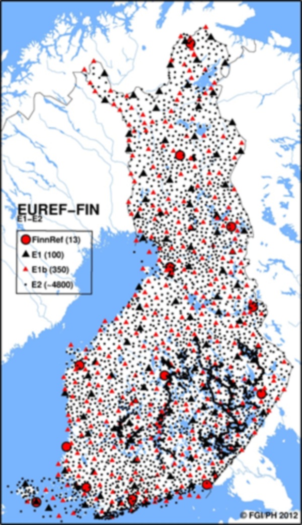
Survey (NLS), for measuring of control points in it. The first order
network (E1), including 12 active FinnRef® GNSS stations and 100 passive
control points, was measured in 1996–97 (Ollikainen et al., 1999 and
2000). E1 defines the EUREF-FIN reference frame. The FGI densified this
network with 350 passive points in 1998–99, and it is classified as E1b
(Ollikainen et al., 2001). The NLS and the Finnish Maritime
Administration have densified these networks with a second order (E2)
passive network that consists of approximately 4,800 points (Figure 1).
The E1-E2 networks constitute a nationwide backbone of passive control
points for EUREF-FIN. In addition to these networks, there are local,
municipality-level, backbone networks (E3-E4) and lower order networks
(E5-E6) for practical daily use.
2.2 Active GNSS networks
Currently, there are three separate networks of
active (permanent, continuously operating) GPS/GNSS stations in Finland.
The Finnish permanent GPS network FinnRef® consists of 13 stations and
is maintained by the FGI (governmental network). FinnRef is the backbone
of the national ETRS89 realization, acting as the link to the
international reference frames through one IGS station (Metsähovi), and
four stations (Metsähovi, Vaasa, Joensuu and Sodankylä) that belong to
the EUREF Permanent Network (EPN). It is also used to connect other
(wide area) active GNSS networks to EUREF-FIN. The time series of the
FinnRef® stations play an essential role in monitoring the stability of
the reference frame, e.g. monitoring the effect of postglacial rebound
in Fennoscandia. FinnRef® is currently being renewed to be GNSS capable
(tracking GPS, GLONASS, Galileo and later also Compass signals) with 19
stations. Most of the old stations will be equipped as dual stations
(with a new monument close to the old one) and the rest of the new
stations will enhance the geometry of the old network (Koivula et al.,
2012).
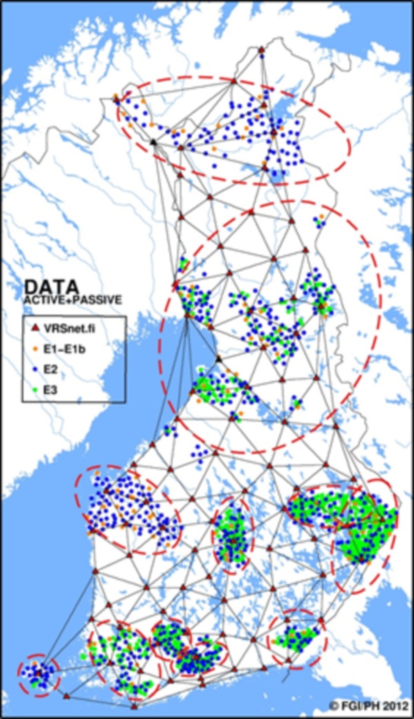
More practical-oriented active networks, such as
network-RTK services, are provided by private companies. In Finland,
there are two network-RTK services available: Trimble-based VRSnet.fi
and Leica-based SmartNet. Geotrim Oy established the VRSnet.fi (formerly
GNSSnet.fi and GPSnet.fi) network in 2000. The network became
operational in 2002–2003, was expanded nationwide in 2005, was upgraded
to GPS+GLONASS in 2006, and later became GNSS capable. The VRSnet.fi
network consists of 88 stations (Geotrim, 2012). Leica Geosystems
started to build the Leica SmartNet network in Finland in 2011.
Currently, the network consists of 58 GNSS stations and, when finished,
it will consist of more than 100 stations covering the whole country
(Leica, 2012). Since the GPS data available for this study were
collected in 2006–2010, we used the VRSnet.fi stations to test the
consistency between active GNSS stations and official passive ETRS89
control points. The network can be seen in Figure 2. The average spacing
of the VRSnet.fi stations is 77 km.
|
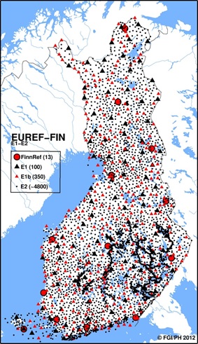
Figure 1. Finnish ETRS89 realization, EUREF-FIN, and its
nationwide densifications (E1-E2). |
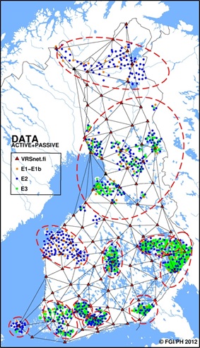
Figure 2. The VRSnet.fi network and the selected test
points for the study. Regional subnets are shown with dotted
lines. |
2.3 GPS data and processing
We have used a set of GPS data collected by the NLS
while doing E2-E3 densification measurements in 11 regions (subnets) in
2006–2010 (Figure 2). Exactly the same data were used to determine the
reference coordinates of the control points in E2-E3. The data also
include observations on fiducial points (E1-E1b points for E2
densifications and E1-E2 points for E3 densifications) since the
original densification measurements were made hierarchically with
respect to the nearest higher order reference points. The study consists
of about 1,450 passive control points in E1-E3 coordinate classes with
an average spacing of 33 km in E1-E1b, 10 km in E2, and 7 km in E3. The
GPS data were processed and adjusted by fixing the active GNSS stations
of VRSnet.fi instead of passive control points. This method neglects the
hierarchy of the control point networks. Since the same GPS data were
originally used for determining the reference coordinates for E2-E3
points, the residuals of this study show explicitly the accuracy of our
alternative, non-hierarchical, method of determining the coordinates for
the points.
The GPS data were processed and adjusted with Trimble
Total Control 2.73 software using double differencing, IGS precise
ephemerides, CODE global ionosphere maps (GIM), 10 degree cut-off angle,
classical Hopfield troposphere model, and otherwise default processing
and adjustment parameters. The data at passive stations were collected
and processed with 15-second observation interval, while active stations
had 30-second observation interval. In total in all subnets, 9,802 and
7,472 baselines (for the network and individual solutions, respectively,
see next paragraph) were processed in the study. The baselines range
from 0.4 km to 260.8 km, the average being 17.8 km for the network
solutions and 51.3 km for the individual solutions. The minimum
occupation time was limited to 30 minutes based on a study by Häkli et
al. (2008), while average occupation times were 2.1 and 2.7 hours for
network and individual solutions. Only baselines with ambiguities
solved/fixed to integers were taken to adjustment.
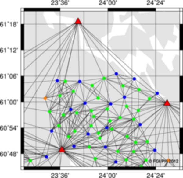
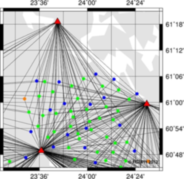
We had two alternative strategies for the
computation. In both cases the coordinates of active VRSnet.fi stations
were kept fixed. In the first solution, all possible baselines were
processed and adjusted together forming closed loop networks in which
most of the baselines between adjacent points were solved (network
solution). The outmost points of the networks were connected to the
nearest active VRSnet.fi stations. In the second solution, the points
were processed and adjusted individually connecting each point only to
the nearest three to four VRSnet.fi stations (individual solution). This
means that inter-point baselines were not solved at all and each point
belongs to its own network. An example of the two cases is shown in
Figure 3.
 |
 |
|
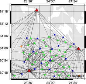
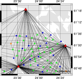
Figure 3. Alternative computation
strategies of the test data. The data were processed as network
(left) and individual (right) solutions. In the network
solutions, adjacent points are mostly tied with a baseline in
between. In individual solutions, all test points were tied only
to the nearest three to four active GNSS stations, leaving the
baselines between the test points unprocessed. |
The two solutions were tested for purposes of
practicality and requests from surveyors. The latter solution strategy
would require only one GNSS instrument (in the field), while the former
solution requires a minimum of two but, in practice, more simultaneously
observing instruments (also considering formation of the loops, trivial
vectors and redundant baselines for the adjustment). This is mainly a
question of cost-effectiveness reducing the required manpower and
investments in instruments.
In both solutions some baselines and points had to be
rejected either after baseline processing or network adjustment. For
example, all float vectors were rejected after baseline processing. The
main reason for rejecting the baselines was insufficient data (too short
occupation time). The test data were originally planned and collected
for hierarchical measurements with relatively short baselines, while the
baselines to the active stations are much longer. As a result, some
baselines with insufficient data exist, especially in individual
solutions where baselines were much longer than in the original
hierarchical measurements. Normally this should be compensated for with
longer occupation times but it was not possible in the case of the
available data. In some cases a baseline rejection led to bad network
geometry, meaning that a point no longer fulfilled the preset
requirement of each point having to be connected with a baseline to at
least three other points. These points had to be eliminated before the
final adjustment. The number of points after the final GPS adjustments
was 1,468 for network solutions and 1,451 for individual solutions.
After successful adjustment the coordinates were compared to the
official EUREF-FIN coordinates of the points. In this paper, we use the
term 'residual' to refer to the difference between the adjusted
coordinates and official coordinates.
3. RESULTS
The residuals were first inspected against outliers.
Since the study period is five years (2006–2010) there are some changes
in instrumentation and reference coordinates in the VRSnet.fi network.
Therefore the outlier analysis was done subnet-wise (same subnets as in
GPS computation that were observed during a relatively short time
period) using three times the standard deviation (3s) as a criterion for
outlier detection. In this case only those points that are inconsistent
with regard to the data set they belong to are rejected. In the residual
analysis 68 and 50 outliers were found for network and individual
solutions, respectively. Most of the outliers are related to the same
reasons as in rejections in GPS processing and adjustment, i.e.
insufficient occupation time for some baseline(s) connected to the
rejected point, bad network geometry or a combination of both. The
rejected points with bad network geometry were mainly points at the edge
of the network, or even outside the VRSnet.fi network at the borders of
Finland, and/or connected to other points asymmetrically.
Proportionally, most outliers were found in the E1
class (12.2/7.1%), while in E2 and E3 the values are 6.3/3.3% and
2.5/3.1%, respectively (for network/individual solutions). A larger
rejection rate in E1 relates to the fact that the reference coordinates
of the E1 points were determined earlier (in 1996–1999) using different
GPS data than what was used in this study, whereas the reference
coordinates of most of the E2 and E3 points were determined with the
same data. The observation epoch difference explains the majority of the
E1 residuals. This is due to, for example, postglacial rebound occurring
in the Fennoscandian area (see more in chapters 4–5). Additionally, the
reference coordinates of the E1 points have been determined using
different instruments, different occupation times, different setups
(e.g. centring and antenna height), different GNSS processing software,
measured under different conditions (e.g. solar activity and satellite
constellation), etc., that cause some discrepancies. There are fewer
rejections in individual solutions but the final number of accepted
points in both solutions is almost the same (1400/1401), which means
that more points in individual solutions were already rejected during
GPS processing and adjustment.
After all precautions taken in GPS processing,
adjustment and outlier detection, an additional investigation into
occupation times was conducted. The baseline lengths were inspected
against occupation times and, in most cases, occupation times were
sufficient regarding the study by Häkli et al. (2008), and therefore
observational accuracy should not play a big role for the coordinate
solutions in this study.
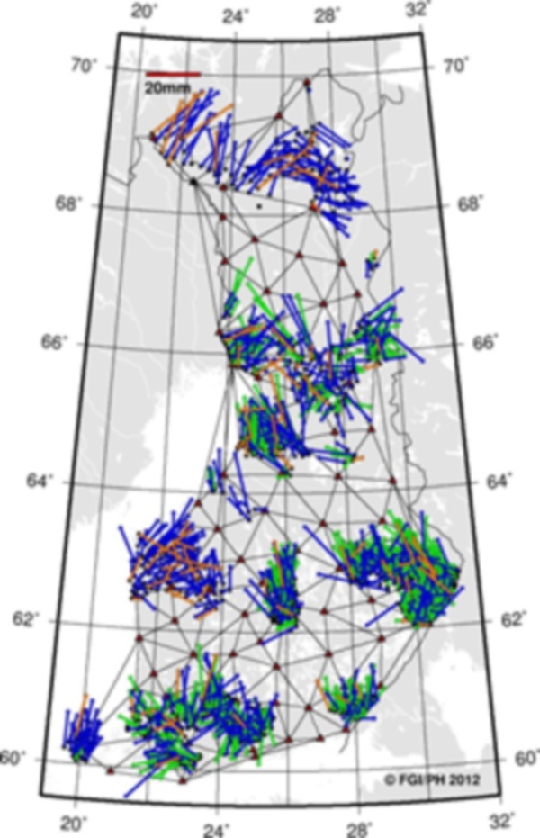
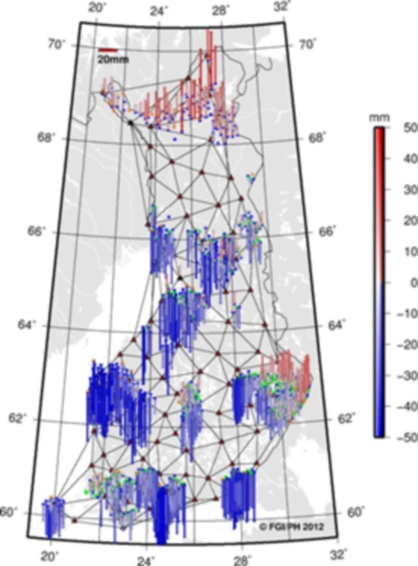
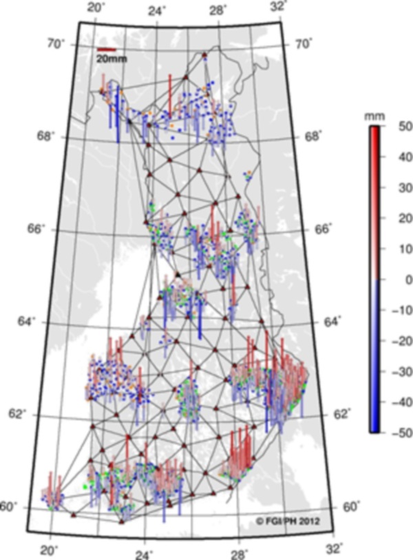
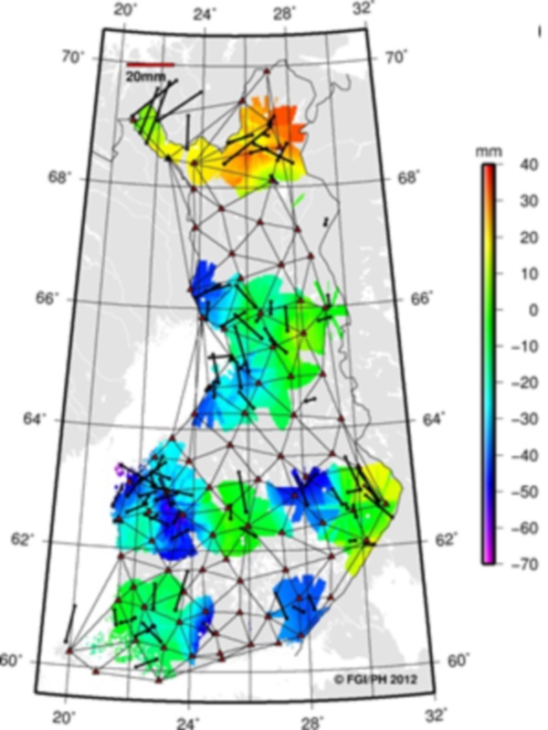
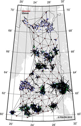
The residuals are summarized in Table 1 for both
solutions after outlier elimination. The results show that two thirds of
static GPS measurements using active stations in both solution types
give roughly an accuracy of 1–3 cm (rms) with respect to the official
passive EUREF-FIN control points. These results sound good for practical
surveying. However, looking at the spatial distribution of the residuals
(Figure 4), it is evident that there are systematic spatial-dependent
residual patterns in both network and individual solutions.
Additionally, considering 95%- or extreme values, the accuracy may not
be enough for all purposes. It is obvious from the figure that residuals
are strongly correlated inside the subnets but less correlated
countrywide. Standard deviation of the residuals is almost doubled from
subnets to countrywide residuals. This and the residual pattern suggest
that the VRSnet.fi network and EUREF-FIN are spatially distorted in
relation to each other. Additionally, the accuracy of the up component
is worse than horizontally by a factor 1:3–4, which is more than typical
(1:2–3) and may imply some biases. In the following sections we analyze
the possible causes for these findings.
Table 1. Statistics of network
and individual solutions after outlier elimination.
| |
Network solution (n=1400) |
Individual solution (n=1401) |
| |
N (mm) |
E (mm) |
U (mm) |
N (mm) |
E (mm) |
U (mm) |
| Min |
-15.40 |
-17.60 |
-79.80 |
-20.90 |
-21.70 |
-73.00 |
| Max |
27.40 |
20.10 |
60.10 |
27.30 |
20.10 |
66.40 |
| Mean |
4.68 |
-0.34 |
-14.32 |
5.10 |
-0.30 |
-13.07 |
| Stdev |
±6.64 |
±6.02 |
±21.09 |
±7.21 |
±6.42 |
±23.55 |
| Rms |
±8.13 |
±6.03 |
±25.50 |
±8.83 |
±6.43 |
±26.93 |
| 95% |
±16.20 |
±12.20 |
±49.20 |
±17.59 |
±13.10 |
±52.00 |
4. ANALYSIS
4.1 Network vs. individual solutions
The effect of the measurement/adjustment technique on
accuracy was tested by solving the point coordinates as networks and
individually from active GNSS stations. The residuals of both solutions
look alike (Table 1 and Figure 4), suggesting that the solution type
would not have a strong effect on accuracy. To see the solution
differences, the solution coordinates were subtracted from each other.
Spatially, the horizontal differences between the solutions are
negligible in most subnets but in the vertical component many subnets
seem to have systematic differences (Figure 5). On the other hand, the
mean difference is less than ±1 mm in each residual component, meaning
that, as a whole, there are non-existent systematic errors between the
solutions (Table 2). The difference in terms of standard deviation, rms
or 95% value is roughly half of the respective values for each solution
in Table 1. On the whole, both techniques perform more or less equally,
showing only a slight advantage to the network solution. However, some
spatial differences in performance between the solutions exist.
 |
 |
|
Figure 5. Difference between the
solutions (individual minus network solution). Horizontal
differences shown on the left and vertical on the right (note
different scale in horizontal and vertical plots). |
Table 2. Difference of
alternative solutions, individual minus network solution.
| |
Individual minus Network solution |
| |
N (mm) |
E (mm) |
U (mm) |
| Min |
-21.70 |
-18.80 |
-64.10 |
| Max |
22.50 |
22.50 |
60.20 |
| Mean |
0.42 |
-0.05 |
0.91 |
| Stdev |
±4.12 |
±3.04 |
±12.67 |
| Rms |
±4.14 |
±3.04 |
±12.71 |
| 95% |
±8.30 |
±6.10 |
±27.20 |
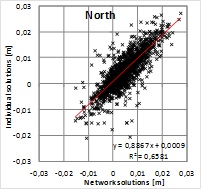
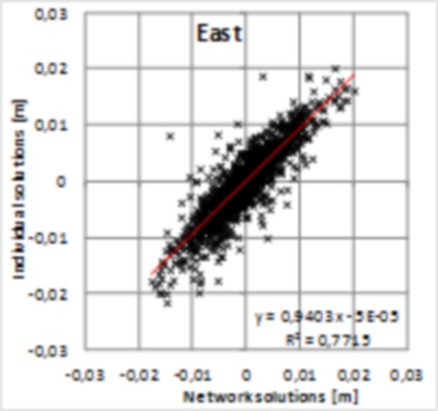
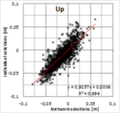
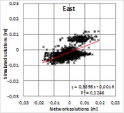
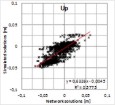
In order to analyze the significance of solution type
for residuals, the solutions are plotted with respect to each other in
Figure 6. Pearson’s correlation coefficient shows a strong correlation
between the solutions giving r=0.81, 0.88 and 0.83 for North, East and
up components, respectively. Squares of correlation coefficients
(R2=0.66, 0.77 and 0.70) indicate that roughly 30% of the residuals
would originate from differences in the solutions and the rest can be
attributed to some common source or sources. This means that majority of
the residual pattern cannot be explained with the solution type. Because
the alternative solutions were computed with the same GPS data and using
the same fixed points, the result indicates that the data and/or the
fixed coordinates may include biases contributing to the residuals more
than the solution type.
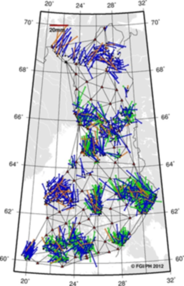
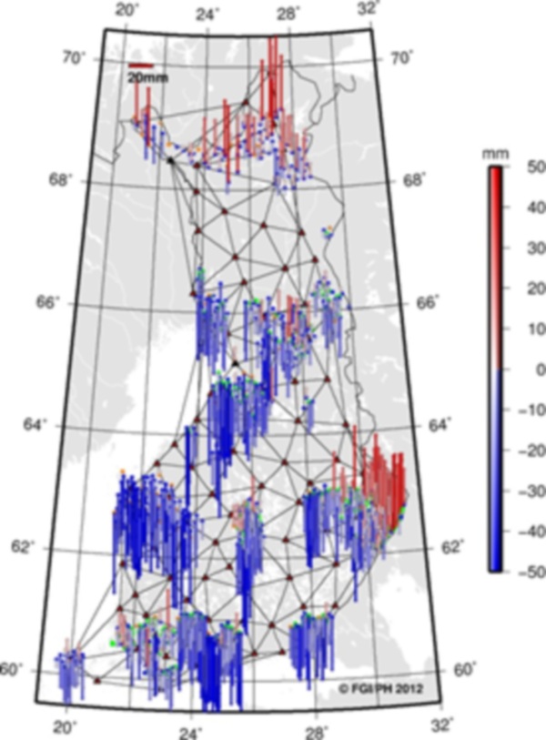
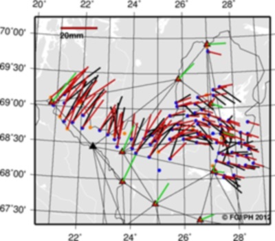
4.2 Agreement between VRSnet.fi and EUREF-FIN
Since no clear distinction could be found between the
solution types, we took the network solutions for further analysis.
Considering the fact that the E1 points have been the reference (fixed)
points in the original EUREF-FIN densifications, and also for the GPS
measurements at E2-E3 points that are used in this study, the residuals
in the E1 points should reveal (at least to some extent and within an
observational accuracy) the differences in the VRSnet.fi network and the
passive control points that define the EUREF-FIN reference frame. To
illustrate the E1 residuals and their possible influence on other
points, the E1 and E2-E3 residuals are plotted separately in Figure 7.
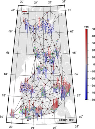
Looking at the horizontal (black vectors) and vertical (colour map)
residuals in the plots, one can instantly see the similarities. This
suggests that most of the residuals seen at the E2-E3 points originate
from E1 or fiducial (VRSnet.fi) points.
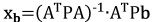
In order to analyse the source of the residuals we
chose a simulation method. In a least squares network adjustment a part
of the observation errors propagates to the residual vector of the
adjustment and a part to the adjusted parameters. If we have systematic
errors in observations, the bias vector propagates to the parameters as
follows:
|
 |
(1) |
|
 |
(2) |
If we assume that only some of the observations have a
bias, then if these observations are stochastically independent of the
other observations having the weight matrix P0 and design matrix A0, we
can study the influence of the bias vector b0 on the parameters without
knowing the other observations. The design matrix in adjustment is:
 |
(3) |
and the weight matrix is
 |
(4) |
resulting in a bias xb to the parameters
 |
(5) |
This was used to study the influence of biased reference
coordinates. Only the network topology from the “from-to” table and the
covariance matrices of the vectors are necessary for the normal equation
matrix. When forming the normal equation matrix (ATPA)–1 the E1
coordinates were first tightly constrained with the covariance matrix
C0. The design matrix A0 includes the identity matrix of size three
times the constrained points. The network geometry and covariance
matrices of baselines were the same as in the case of the network
solution. No actual coordinate difference observations (i.e.
measurements) were used because only the normal equation matrix but not
the normal equation vector was needed. While in GPS processing and
adjustment the coordinates of the active VRSnet.fi stations were kept
fixed, here we did the opposite by constraining the coordinates of the
passive E1 points and calculated the influence of the bias, xb to the
other points including E2-E3 points and the VRSnet.fi stations as well.
The bias in the fiducial coordinates was taken from the E1 residuals of
this study (adjusted minus the official reference coordinates).
 |
 |
|
Figure 7. Residuals between coordinate
classes. E1 residuals shown on the left and E2-E3 on the right.
Horizontal residuals shown with black vectors and vertical with
color map. |
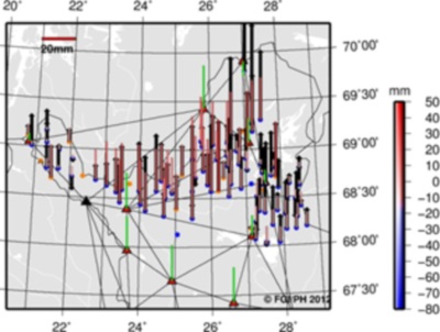
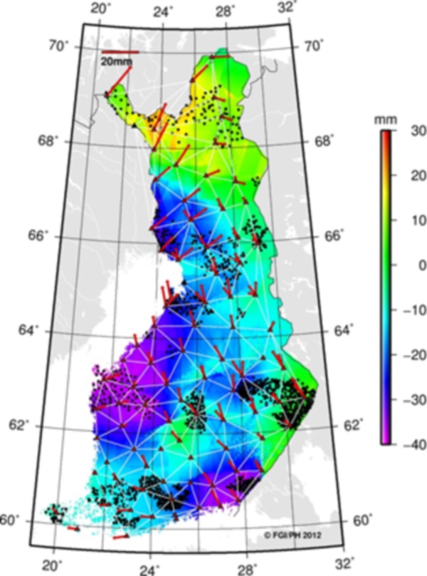
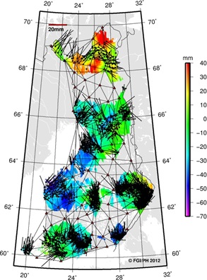
The simulated biases can be analyzed twofold: how the
residuals at E1 points propagate to lower order points and, if the E1
residuals originate from the VRSnet.fi network, how large the biases
would have to be at the active stations. The former can be used to weigh
the significance of the simulated biases by comparing them to the
residuals of the network solutions at E2-E3 points. The latter indicates
the accuracy of VRSnet.fi coordinates in EUREF-FIN reference frame (that
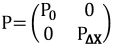
is defined by E1 points). A snapshot of the simulated biases (also at
the VRSnet.fi stations) together with the residuals is plotted in Figure
8. The simulated biases and residuals look alike, suggesting that the
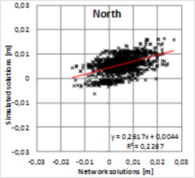
method predicts residuals fairly well. Figure 9 shows the countrywide
correlation between the simulations and the network solutions.
Considering the correlation, there were three subnets with only one E1
point, meaning that the residual is propagating as such to the other
points. These subnets together with the E1 points (at which the
correlation is 1) were removed from the correlation analysis. Medium or
strong correlation (r=0.48, 0.57 and 0.76) was found for North, East and
up components, respectively. Considering the smaller size of the
horizontal residuals compared to the vertical residuals, non-existent
observation errors in simulations and R-squared values (R2=0.23, 0.32
and 0.58) between simulation and network solution, this result suggests
that observation errors dominate the horizontal residuals between E1 and
E2-E3 points but a large part of the vertical residuals at E2-E3 points
would originate from the E1 residuals.
 |
 |
|
Figure 8. Snapshot of comparison of
network and simulated solutions. On the left horizontal and on
the right vertical residual (note different scale). Black
vectors indicate residuals from the network solution and red or
colored vectors are simulated residuals. Simulated residuals for
VRSnet.fi stations are shown with green vectors. A black
triangle indicates one VRSnet.fi station from where the data
were unavailable for the study period.
|
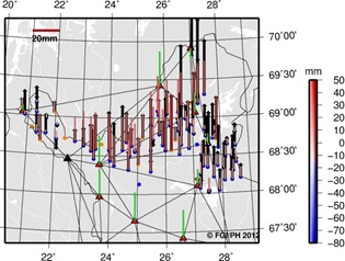
Considering the fairly good predictability for E2-E3
points and reflecting this result on the simulated biases at the
VRSnet.fi stations, they would suggest that the biases can be considered
more significant in the vertical component but less so in the horizontal
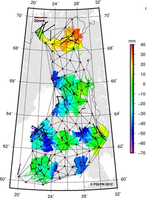
part. The simulated biases for VRSnet.fi stations are shown in Figure 10
(results from the three subnets with only one E1 station not shown
here). Some stations have more than one bias because they have been
fiducial stations in more than one subnet. Most of the multiple biases
for a station are fairly equal, suggesting good compatibility. The
simulated biases show that the agreement between VRSnet.fi stations and
EUREF-FIN is in the order of 5–10 mm in horizontal and 25 mm in vertical
coordinates (rms).
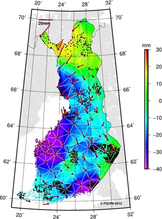
Figure 10. Simulated biases for
the VRSnet.fi stations. The biases can only be considered as indicative.
If the station has more than one bias, it has been a fiducial station in
more than one subnet.
Assuming the simulations are reliable, this could be
considered a good result for the horizontal part but some improvements
could be made for the vertical coordinates. This discrepancy however,
can only be considered as an implication of disagreement due to, for
example, extrapolation of the biases, and it can be interpreted as a
bias in the reference frame, coordinates of the VRSnet.fi or a
combination of both. The most likely reason for the disagreement is the
postglacial rebound (PGR) phenomenon occurring in the Fennoscandian
area, which is deforming the crust of the Earth (e.g. see papers by
Milne et al. (2001) and more recent papers by Lidberg et al. (2007) and
(2010)). The PGR mostly influences vertical coordinates (from a couple
of millimeters to about one centimeter per year in Finland) but has a
small horizontal component as well (up to a few millimeters a year).
Considering the effect and that the reference epoch of the EUREF-FIN is
1997.0, it is obvious that the precision of the frame has degraded since
its realization. This was also shown in a paper by Häkli and Koivula
(2012). However, even if some implications of the reference
frame-related issues were found, it is not the subject of this study. A
more thorough investigation on the coordinates of the VRSnet.fi network
is needed to draw firmer conclusions and to confirm that the residuals
are caused by the uplift phenomenon.
5. CONCLUSIONS AND DISCUSSION
We have studied the accuracy of static GPS surveying
using active GNSS stations with respect to the official hierarchical
passive control point networks that, in Finland, define the ETRS89
realization, EUREF-FIN. The study shows that ignoring the coordinate
hierarchy results in an accuracy (rms) of approximately 1 cm in
horizontal and 2–3 cm in the vertical coordinates. The result is
probably enough for most purposes but it includes, however, some
systematic features, especially in vertical coordinates, and it could be
improved by correcting for the biases. Our analysis implies that a part
of the biases would be caused by distortions between the active
VRSnet.fi network and the passive EUREF-FIN reference frame.
The Earth is constantly changing and the major
challenge in maintaining accurate (static) reference frames in Finland
is the postglacial rebound that deforms the control point networks.
While in the past the traditional measurements were made hierarchically
in a smaller area and relative to the nearest control points together
with a lower quality, this disagreement did not play a role for several
decades from the realization. With current (GNSS) techniques the issue
appears sooner, especially for wider areas, due to more homogeneous and
improved observation accuracy. Our analysis (still inconclusive on the
matter) implies also that postglacial rebound has an influence on the
accuracy of this study. Similar results were reported for virtual data
generated from the same VRSnet.fi network in Häkli (2006). It is obvious
that the determination of ETRS89 coordinates for (wide) active GNSS
networks needs more consideration in the future. Currently, there are
on-going discussions on how this effect should be dealt with. Some
possible solutions are already available, such as the solution
introduced by the Nordic Geodetic Commission (NKG) that includes
transformation formulae and a model correcting for intraplate
deformations caused by postglacial rebound (Nørbech et al. 2008). For
Finland, this approach was evaluated in a paper by Häkli and Koivula
(2012) that verifies this deformation has to be taken into account in
order to reach centimeter level accuracies. Even if some implications of
reference frame-related issues were found, it is not a subject for this
study and so it was not investigated further.
We also studied whether the adjustment strategy has
an influence on accuracy. We computed two alternative solutions where,
in the first solution, baselines were processed and adjusted as closed
loop networks (network solution), while in the other solution each point
was connected to only the nearest three or four active GNSS stations
without processing the baselines between the points at all (individual
solution). The results show that in our study the solution strategy does
not play a significant role in the obtained accuracies. However, one
must remember that measuring control points individually and fixing them
only to active stations may destroy the relative accuracy between the
neighboring points. This will probably not be a problem if the spacing
between the points is large enough but, for example, considering the
accuracies of this study, rms of ±25 mm for the up component means that
a relative error between the points can be 50 ppm for a 1 km baseline.
Therefore it may still be prudent to measure the baselines between the
points if the inter-point distance is small or if good accuracy with
high confidence is required.
REFERENCES
Geotrim (2012). VRSnet.fi webpage:
http://www.geotrim.fi (accessed
30.9.2012)
Häkli, P. (2006). Quality of Virtual Data Generated
from the GNSS Reference Station Network. Shaping the Change, XXIII FIG
Congress, Munich, Germany, October 8–13, 2006. 14pp.
Häkli, P. and H. Koivula (2012). Transforming ITRF
Coordinates to National ETRS89 Realization in the Presence of
Postglacial Rebound: An Evaluation of Nordic Geodynamical Model in
Finland. In Kenyon et al. (Eds.): Geodesy for Planet Earth: Proceedings
of the 2009 IAG Symposium, Buenos Aires, Argentina, 31 August – 4
September 2009. International Association of Geodesy Symposia, 136,
2012, DOI: 10.1007/978-3-642-20338-1.
Häkli, P., H. Koivula ja J. Puupponen (2008).
Assessment of practical 3-D geodetic accuracy for static GPS surveying.
Integrating Generations, FIG Working Week 2008, Stockholm, Sweden 14–19
June 2008. 14pp.
Koivula, H., J. Kuokkanen, S. Marila, T. Tenhunen, P.
Häkli, U. Kallio, S. Nyberg, and M. Poutanen (2012). Finnish Permanent
GNSS Network. Proceedings of the 2nd International Conference and
Exhibition on Ubiquitous Positioning, Indoor Navigation and
Location-Based Service (UPINLBS 2012), 3–4 October 2012, Helsinki,
Finland. IEEE Catalog Number: CFP1252K-ART. ISBN: 978-1-4673-1909-6.
Leica (2012). Leica SmartNet web pages
http://fi.smartnet-eu.com (accessed 30.9.2012)
Lidberg, M., J.M. Johansson, H.-G. Scherneck and J.L.
Davis (2007). An improved and extended GPS-derived 3D velocity field of
the glacial isostatic adjustment (GIA) in Fennoscandia. Journal of
Geodesy, 81, 2007, 213–230. DOI 10.1007/s00190-006-0102-4.
Lidberg, M., J.M. Johansson, H.-G. Scherneck, and
G.A. Milne (2010). Recent results based on continuous GPS observations
of the GIA process in Fennoscandia from BIFROST. Journal of Geodynamics,
50:1, 2010, 8–18. doi:10.1016/j.jog.2009.11.010.
Milne, G. A., J. L. Davis, J. X. Mitrovica, H.-G.
Scherneck, J. M. Johansson, M. Vermeer, H. Koivula (2001).
Space-Geodetic Constraints on Glacial Isostatic Adjustments in
Fennoscandia. Science 291, 2381–2385.
Nørbech, T., K. Engsager, L. Jivall, P. Knudsen, H.
Koivula, M. Lidberg, B. Madsen, M. Ollikainen, M. Weber (2008).
Transformation from a Common Nordic Reference Frame to ETRS89 in
Denmark, Finland, Norway, and Sweden – status report. In Knudsen, P.
(Editor): Proceedings of the 15th General Meeting of the Nordic Geodetic
Commission, Copenhagen, Denmark, May 29 – June 2, 2006. Technical Report
No. 1, National Space Institute, 102–104. ISBN 10 87-92477-00-3.
Ollikainen, M., H. Koivula ja M. Poutanen (1999). The
Densification of the EUREF Network in Finland. IAG, Section I –
Positioning, Commission X – Global and Regional Geodetic Networks,
Subcommission for Europe (EUREF). Report on the Symposium of the IAG
Subcommission for Europe (EUREF) held in Prague, 2–5 June 1999.
Veröffentlichungen der Bayerischen Kommission für die Internationale
Erdmessung, Heft 60, 114–122. München.
Ollikainen, M., H. Koivula ja M. Poutanen (2000). The
Densification of the EUREF Network in Finland. Publications of the
Finnish Geodetic Institute N:o 129. Kirkkonummi 2000. ISBN
951-711-236-X.
Ollikainen, M., H. Koivula ja M. Poutanen (2001).
EUREF-FIN-koordinaatisto ja EUREF-pistetihennykset Suomessa.
Geodeettisen laitoksen tiedote 24. ISBN 951-711-243-2.
BIOGRAPHICAL NOTES
Pasi Häkli and Ulla Kallio are research scientists
(M.Sc. Tech.) at the Finnish Geodetic Institute. Jyrki Puupponen is a
cartographic engineer (M.Sc. Tech.) at the National Land Survey of
Finland.
CONTACTS
Pasi Häkli and Ulla Kallio
Finnish Geodetic Institute
Department of Geodesy and Geodynamics
P.O. Box 15
FI-02431 Masala
FINLAND
Email: pasi.hakli@fgi.fi,
ulla.kallio@fgi.fi
Web site: http://www.fgi.fi
Jyrki Puupponen
National Land Survey of Finland
South Finland District Survey Office
P.O. Box 11
FI-15141 Lahti
FINLAND
Email:
jyrki.puupponen@maanmittauslaitos.fi
Web site:
http://www.maanmittauslaitos.fi/
 |